
Geotechnical engineering libraryContact
 benesch
Geotechnical Services Manual for Railroad Clients
A Consultant's Reference for Delivering Geotechnical Engineering Services Across North American Railroad Capital Programs
Apps on dirtbert.com that support this chapter. Each one runs in a web browser on a desktop or a phone, with nothing to install. How to use the apps (I.3). Tools marked TOOLS open in the Geotechnical Analysis Suite (Benesch sign-in); the orange card below lists each one by section.
NANCY pages ask you to accept the Use and Disclaimers once in each browser. MINA is a monitoring aid and is not for operational dispatch decisions.
Calculators and workbook tools from the Benesch Geotechnical Analysis Suite that support this chapter: 3 interactive calculators and 5 workbook guides. Each one is also placed inside the section it supports, in an orange tools strip.
| FF | Field Observation DataUsed in 15.6 Settlement Monitoring | Calculator ▸ | Guide |
| FF | Dynamic Cone Field LogUsed in 15.2 Compaction Testing | Calculator ▸ | Guide |
| PV | FAA P-501 Random SamplingUsed in 15.2 Compaction Testing | Calculator ▸ | Guide |
| FF | Daily Log — Compaction Testing (Nuclear Gauge)Used in 15.2 Compaction Testing | guide only | Guide |
| DF | CSL Analysis (Crosshole Sonic Logging)Used in 15.4 Pile Installation Monitoring | guide only | Guide |
| DF | Pile PDA Field Data ComputationsUsed in 15.4 Pile Installation Monitoring | guide only | Guide |
| DF | Pile Load Test Calculations (Compression)Used in 15.5 Static Axial Load Testing (ASTM D1143) | guide only | Guide |
| FF | Nuclear Density — SoilUsed in 15.2 Compaction Testing | guide only | Guide |
Tools open on dirtbert.com and need the Benesch sign-in. Drafts pending Benesch final review, not for use in design.
General topic illustrations from Benesch's shared geotechnical graphics library, related to this chapter's subject matter — not the numbered figures called out in the text above. Click any image to view it full size.
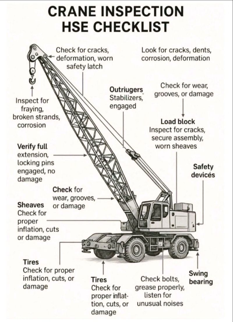
Construction monitoring is the geotechnical consultant's final opportunity to verify that subsurface conditions match design assumptions, that materials meet specification, and that construction methods produce the intended product. In railroad capital programs, the consequences of failed construction QA are measured not only in dollars but in operational downtime, derailment risk, and long-term maintenance cost. A well-designed embankment that is poorly compacted will fail progressively. A pile that is driven through the wrong soil horizon will under-perform. A staged embankment advanced too quickly will trigger slope failure.
This chapter covers the full scope of construction-phase geotechnical services delivered to all nine client railroads: compaction testing (nuclear gauge and sand cone methods), proof rolling, pile installation monitoring (WEAP, PDA, CAPWAP), static axial load testing, settlement monitoring (settlement plates and survey), piezometric monitoring during staged construction, inclinometer monitoring for slope and wall movements, trigger levels and action plans, and construction QA/QC documentation. All test methods are referenced to current ASTM standards. Client-specific inspection and reporting requirements are tabulated for all nine railroads.
The correlations below are used or referenced in this chapter. Each is a statistical fit to a particular data set, so a value from one is an estimate: it applies only within the materials and ranges stated, carries the scatter of the original data, and must be confirmed by site-specific testing or calibration before it is relied on for design.
When an equation is used, note it with the result: give the equation ID and source, state that the soil or rock is within its range of applicability, mark the value as correlated (not tested), and record the limitation that governs. The Empirical Equations & Correlations reference has every entry with its full references.
Variables. Nm = field blow count; ERm = measured hammer energy ratio (%); CB = borehole diameter (1.0 for 65–115 mm, 1.05 for 150 mm, 1.15 for 200 mm); CS = sampler (1.0 standard, 1.1–1.3 liner-less); CR = rod length (0.75 <3 m; 0.8 3–4 m; 0.85 4–6 m; 0.95 6–10 m; 1.0 >10 m)
Use. All soils tested by SPT (ASTM D1586). Normalizes blow count to 60% of theoretical free-fall energy, the basis for most U.S. correlations.
Limitations. CE ranges ~0.5–1.6 depending on hammer type; use measured energy (ASTM D4633) where available. Rod-length factor ranges differ between Skempton (1986) and Youd et al. (2001).
Source. Skempton 1986; Youd et al. 2001 · In this chapter: 15.4 · Full entry and references
Variables. Cα = Δe / Δlog t
Use. Secondary consolidation of soft soils; the ratio holds at a given effective stress level.
Limitations. Use Cc corresponding to the final stress (Cc varies with stress in structured clays).
Source. Mesri & Godlewski 1977; Mesri & Castro 1987 · Full entry and references
Variables. u2 = pore pressure behind cone tip; an = net area ratio (typically 0.70–0.85, from calibration)
Use. All piezocone (CPTu) soundings; essential in soft clays and silts.
Limitations. Correction negligible in clean sands; critical in soft fine-grained soils. Requires u2 filter position.
Source. Lunne et al. 1997 · Full entry and references
Variables. k = empirical factor
Use. Intact, inorganic clays.
Limitations. k is higher in aged/heavily OC clays and lower in fissured clays; calibrate with oedometer tests.
Source. Kulhawy & Mayne 1990; Mayne 1995 · Full entry and references
Railroad construction monitoring differs from typical civil construction monitoring in three critical ways:
ASCE Manual 73 (ASCE 2012) separates two functions that are often blurred together as “QA/QC.” Quality assurance is the planned, systematic work of the owner or its agent to gain confidence that the design complies with codes and criteria and that construction complies with the contract documents; it verifies that the other parties’ quality control is working. Quality control belongs to the design professional (control of the contract documents) and to the constructor (control of the work), and includes observations, calculations, inspections, tests and documentation.
The owner sets the value placed on quality, funds it, and decides whether to use a standing generic QA plan, a project-specific plan, or a tailored generic plan. The owner may specify the designer’s and constructor’s QC plans prescriptively or in performance terms. During construction the owner must choose who inspects: the owner, the design professional, an independent agency, a code official, or the constructor. The Manual stresses that none is always best and the choice should balance cost, safety, schedule and quality. A resident project representative (RPR) may oversee the constructor’s QC and reviews the constructor’s QC plan before production starts.
A typical constructor project-specific QC plan addresses a skilled workforce, a QC organization, a submittal schedule, inspections, mock-ups and sample construction, a testing plan including special inspections, documentation, and corrective action when acceptance criteria are not met. It should also cover subcontractor qualification, control of measuring and test equipment, and segregation of nonconforming material. The Manual summarizes responsibilities in a chart: the owner establishes the QA program; the designer develops design-phase QC; the constructor develops and documents construction QC; and all communicate regularly.
For railroad work: On a railroad-funded embankment or subgrade project the railroad (or its engineering consultant acting as RPR) performs QA, and the contractor performs QC testing such as compaction and gradation. When the geotechnical consultant’s field staff perform acceptance testing, the scope should say whether that testing is QA (owner verification) or is replacing contractor QC, because the two carry different responsibility for rework and different testing frequencies. State this explicitly in the construction monitoring scope and the GSP.
Source: American Society of Civil Engineers (2012). Quality in the Constructed Project: A Guide for Owners, Designers, and Constructors, 3rd ed. ASCE Manuals and Reports on Engineering Practice No. 73. Reston, VA: ASCE, pp. 169–170, 191–199. Summarized and paraphrased. Full reference under Supplemental Sources.
Compaction acceptance is based on relative compaction (RC) referenced to the laboratory maximum dry density (MDD):
RC = (γ_d,field / γ_d,max) × 100%
where:
All nine client railroads specify Modified Proctor (ASTM D1557) as the reference for embankment, blanket layer, and subballast compaction. Standard Proctor is used only for structure backfill behind retaining walls at G&W (per G&W Engineering Bulletin).
Client compaction requirements (from Chapter 18, Table 10-7, restated here for construction context):
| Railroad | Min. RC (Subgrade/Blanket) | Min. RC (Embankment) | Test Method | Governing Std. |
|---|---|---|---|---|
| CSXT | 95% | 90% | ASTM D6938 (nuclear) | CSXT Eng. Std. Sec. 7 |
| NSR | 95% | 90% | ASTM D6938 or D1556 | NSR Eng. Std. Sec. 7 |
| G&W | 95% | 90% | ASTM D6938 or D1556 | G&W Eng. Bulletin |
| UPRR | 95% | 92% | ASTM D6938 | UPRR Eng. Instr. Manual |
| BNSF | 95% | 92% | ASTM D6938 | BNSF Eng. Instructions |
| CPKC | 95% | 90% | ASTM D6938 | CPKC Track Standards |
| Amtrak | 95% | 92% | ASTM D6938 or D1556 | Amtrak Eng. Std. |
| CN | 95% | 90% | ASTM D6938 | CN Eng. Standards |
Reference graphics
The nuclear gauge measures in-place density and moisture content using a radioactive source (cesium-137 for backscatter; americium-241/beryllium for direct transmission). The gauge reports:
γ_d,field = (WD - count ratio correction) × calibration constant (pcf)
In practice, results are read directly from the calibrated gauge display. Field procedure:
Gauge calibration: ASTM D6938 requires calibration on a reference block before each use. Nuclear gauges are licensed NRC devices; technician must hold current radiation safety training certification. All nine client railroads require gauge operators to carry their radiation license during field work.
Gauge correction for materials containing significant gravel or rock: ASTM D6938 permits an oversize correction when more than 30% of material is retained on the ¾-in. sieve:
γ_d,corrected = γ_d,gauge + [(G_c − G_s) × P_c × γ_w] (pcf)
where G_c = specific gravity of coarse fraction; G_s = average specific gravity assumed by gauge; P_c = fraction coarser than ¾ in.
The sand cone method is required by NSR, Amtrak, and G&W for acceptance testing in compacted structural fill adjacent to structures and retaining walls, and as the verification method when nuclear gauge results are disputed.
Field bulk density:
ρ_bulk = (M_soil) / V_hole (pcf)
Volume of hole:
V_hole = (M_cone−sand,initial − M_cone−sand,final − M_sand,funnel) / ρ_sand,calibrated (ft³)
Dry density:
γ_d = ρ_bulk / (1 + w/100) (pcf)
where w = gravimetric water content (%) from oven-dried sample (ASTM D2216).
Sand cone testing is slower than nuclear gauge but is considered the more accurate reference method. Minimum test frequency: 1 test per 500 cy compacted fill per NSR; 1 per 1,000 cy per CSXT.
Reference graphics · click to zoom
| Application | Frequency | Trigger for Retest |
|---|---|---|
| Embankment lift (main body) | 1 test per 500 ft of track per lift | RC < minimum |
| Blanket layer / subgrade prep | 1 test per 250 ft of track per lift | RC < minimum |
| Structural fill (bridge abutment) | 1 test per 2 ft lift per 50 ft length | RC < minimum |
| MSE wall reinforced fill | 1 test per 2 ft lift per 100 ft | RC < minimum |
| Retaining wall backfill | 1 test per 2 ft lift per 50 ft | RC < minimum |
| Trench backfill (pipe, drain) | 1 test per 50 linear ft per lift | RC < minimum |
Source: Compiled from CSXT Eng. Std. Sec. 7, BNSF Eng. Instructions, NSR Eng. Std. Sec. 7, AREMA MRE Ch. 1.
The purpose of compaction is to gain strength and stiffness, reduce compressibility, plastic strain under repeated load, permeability and swell. Density is just the convenient thing to specify. Keep these points in mind when setting and checking specifications:
After Selig & Waters (1994), chs. 9 and 11. Full reference under Supplemental Sources.
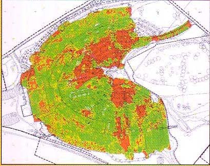
Spot tests sample a tiny fraction of a lift. Roller-integrated measurement covers 100% of the area and can find soft zones deeper than a nuclear gauge. SHRP2 distinguishes CCC (the roller records a drum-response stiffness value with GPS position) from intelligent compaction (the roller also adjusts amplitude, frequency or speed automatically). It is best suited to granular fills, sand, crushed gravel and rock fill — i.e., subballast and embankment granular layers. The Austrian contractual provisions summarized by Adam (2007) show how to make it an acceptance test:
A falling roller value on repeated passes indicates loosening, particle crushing or pore pressure build-up — a reason to stop rolling, not to add passes.
Source: Adam, D. (2007). “Roller-integrated Continuous Compaction Control (CCC): Technical Contractual Provisions & Recommendations.” In Gomes Correia, A., Momoya, Y. and Tatsuoka, F. (eds.), Design and Construction of Pavements and Rail Tracks. Taylor & Francis/Balkema · SHRP2 R02 / GeoTechTools (2012). Intelligent Compaction — technology fact sheet
UIC practice compacts the formation layer (the improved top-of-subgrade layer over S1 or S2 subsoil) to 100% of Standard Proctor, compared with 95% routinely specified for embankment subsoil. The formation layer also has to be homogeneous, without local concentrations of fine material, and placed on subsoil with a low water content. Otherwise subsoil fines migrate into it and the 3–5% crossfall is lost. Field QA should therefore watch uniformity and subsoil moisture as well as density.
After Profillidis (2014), §9.7.1. Full reference under Supplemental Sources.
Profillidis sets two checks before track laying begins: the subgrade has been properly compacted, and the 3–5% crossfall is correctly formed. Ballast is then delivered by special wagons, placed, levelled, graded and consolidated with a vibrating plate or roller. Uniform tie spacing matters as much as the nominal spacing. A high-speed laying machine averages about 0.81 mi per 6-hour shift, with peaks of 1,640 ft/h and 0.93–1.2 mi per shift. Once laid, the rails are set with a rail-positioning machine (Figure 15-11).
For the geotechnical inspector, those two checks are natural hold points. Document the subgrade density results and a crossfall survey before the contractor places ballast, because neither can be corrected afterward without removing the track.
Figures · click to zoom
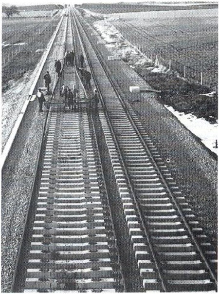
After Profillidis (2014), §16.1.1, Fig. 16.1. Full reference under Supplemental Sources.
Backfill and compact every 2-ft lift; skipped lifts leave voids that resettle under traffic. Match the compactor to the soil: a smooth-drum vibratory roller for granular fill, and never a sheepsfoot on saturated silt or clay, which can liquefy. Excavate in lifts and shore or slope trenches; trench collapses kill roughly 50 people a year in Canada. Wear rain gear and keep clear of live track when digging beside the rail.
Figures · click to zoom
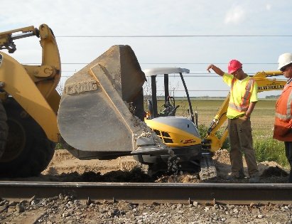
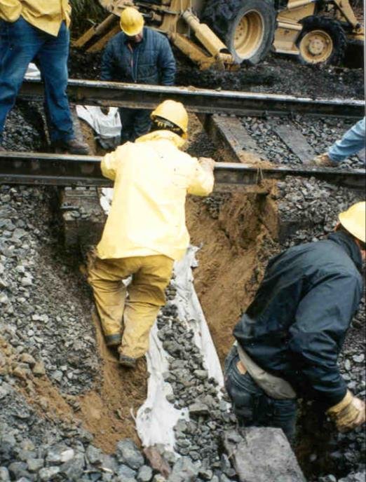
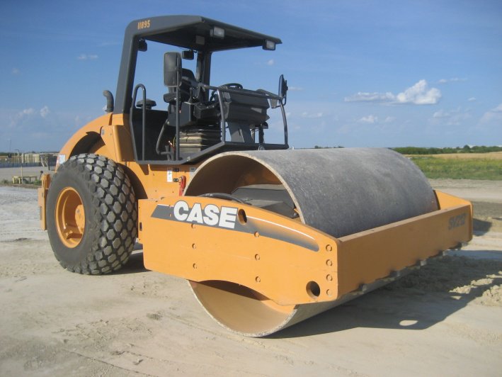
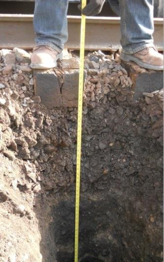
After Geotechnology for Railroaders Program, Module 6.2, Module 6.1; Module 6.2 §02, §05; Module 6.1 §02. Full reference under Supplemental Sources.
Case study: 15.18.1 Field moisture ratios behind 5,649 passing density tests (Look 2023), in §15.18 Case Studies.
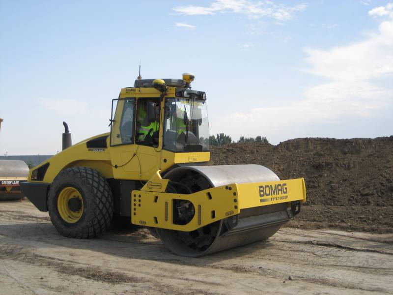
Proof rolling is a rapid field technique for identifying soft, pumping, or inadequately compacted subgrade zones prior to placing overlying layers. It is required by CSXT, NSR, UPRR, and BNSF for all mainline subgrade preparation.
Method: A loaded dump truck (minimum 25-ton axle load, or loaded hi-rail tanker as approved) traverses the prepared subgrade at 2–3 mph. The geotechnical inspector observes for:
Reporting: GPS-tagged station of each deficiency location. Soft areas are marked, overexcavated to competent material (confirmed by nuclear gauge or hand penetrometer), and replaced with approved compacted fill.
Limitation: Proof rolling detects near-surface softness (top 18–24 in.) only. It does not evaluate deeper consolidation or deep subgrade conditions. Supplement with nuclear gauge density testing.
Reference graphics
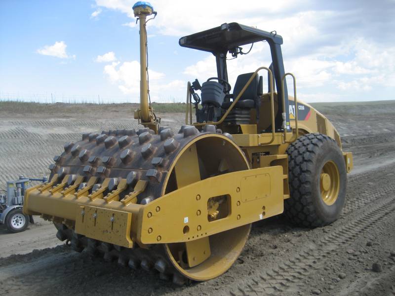
Reference graphics · click to zoom
Inspect the subgrade at every stage of preparation, and again just before geotextile or sub-ballast is placed. Once the subgrade is covered, problems are expensive to find and fix.
| Item | Requirement | Inspector check |
|---|---|---|
| Subgrade | Inspected at each stage of preparation and before geotextile or sub-ballast is placed | Proof roll (§15.3); record stations of soft areas and repairs |
| Drainage | Ditches, culverts, subdrains and nearby earthwork complete before final subgrade preparation | Inspect subdrains before covering; check ditch flow lines and sections before track work starts |
| Geotextile exposure | No more than 7 days from removal of the shipping cover to final placement | Record delivery and uncovering dates in the daily field report |
| Geotextile cover | No equipment on geotextile until it has at least 6 in. of sub-ballast or ballast cover | Stop equipment tracking onto exposed fabric |
| Geotextile overlap | At least 3 ft, longitudinal and transverse | Measure at each seam |
| Geotextile contamination | Surface drainage directed away from placed fabric | Check for silted or blinded fabric before covering |
| Sub-ballast | Placed to plan lines and grades; compacted to at least 95% of ASTM D1557 (modified Proctor) maximum dry density | Test at the Table 15-1 frequency; check grade |
| Ballast placed by truck | No rutting that blocks drainage of sub-ballast or subgrade | Level and grade any ruts to drain before more ballast is placed |
Ballast delivery. For large quantities (several hundred tons or more), unloading from ballast hopper cars is usually the most efficient method. Where the owner has a locomotive and crew, using them to spot ballast cars for the contractor can lower the unit cost. Settle that arrangement in the contract documents and at the pre-construction meeting. Where trucks place ballast, watch for rutting: ruts in sub-ballast or subgrade hold water under the track.
After UFC 4-860-01FA (2004), ch. 9, §4 and §5a, 5c. Full reference under Supplemental Sources.
Reference graphics
WEAP is a predictive analysis performed before driving to establish the driving criterion (blow count per foot at target penetration depth or refusal) that corresponds to the required pile capacity. It models the pile, hammer, and soil system using wave propagation theory.
WEAP output:
Hammer energy — English units:
E_rated = W_ram × h (ft·lb)
where:
Transferred energy:
E_transferred = F_max² × L_pile / (2 × E_pile × A_pile) (ft·lb, from wave equation solution)
Required input parameters for WEAP:
Smith damping constants (typical):
| Soil Type | Side Quake (in.) | Tip Quake (in.) | Side Damping (s/ft) | Tip Damping (s/ft) |
|---|---|---|---|---|
| Sand | 0.10 | 0.10 | 0.05 | 0.15 |
| Clay | 0.10 | 0.10 | 0.20 | 0.15 |
| Silt | 0.10 | 0.10 | 0.15 | 0.15 |
WEAP is required by UPRR and BNSF Engineering Instructions for all bridge foundation piles; by CSXT and NSR for piles > 60 ft length or in soft clay.
Values from these correlations are estimates, not test results. State the equation ID and source when one is used, confirm the soil or rock is within its range, and calibrate against site testing before design.
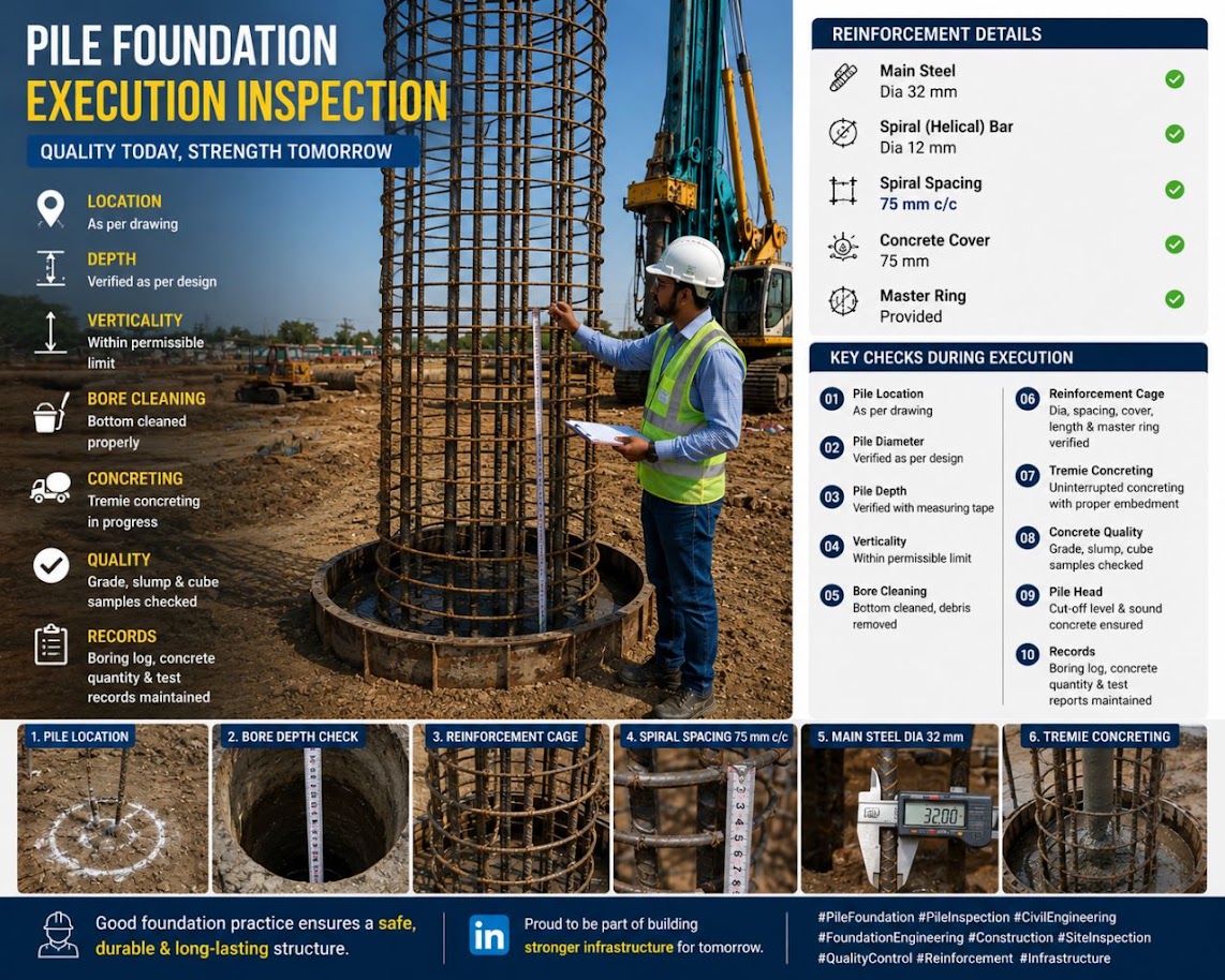
The PDA measures force and velocity at the pile head during driving using strain gauges and accelerometers. It provides a real-time assessment of:
Case Method capacity:
R_total = ½ × (1 + J_c) × [F(t₁) + Z × V(t₁)] + ½ × (1 − J_c) × [F(t₁ + 2L/c) + Z × V(t₁ + 2L/c)] (lb)
where:
Transfer ratio: ETR = (E_transferred / E_rated) × 100%. Per UPRR and BNSF requirements: ETR ≥ 60% for hydraulic hammers; ETR ≥ 40% for diesel.
Minimum PDA testing frequency:
CAPWAP (CAse Pile Wave Analysis Program) is a post-processing signal matching analysis of PDA records that provides:
CAPWAP replaces WEAP as the definitive capacity prediction when PDA data is available. All nine client railroads accept CAPWAP results as equivalent to 1 static load test when performed on ≥ 2% of production piles with approved restrike protocol (restrike after minimum setup time: 24 hours in sand; 7 days in clay).
Source: U.S. Army Corps of Engineers (1997). Pile Driving Equipment. Engineering Instructions EI 02G001 · Swan, C. C. Field Estimates of Pile Capacities, 53:139 Foundation Engineering supplemental notes. The University of Iowa · Hannigan, P. J. et al. (2006). Design and Construction of Driven Pile Foundations. FHWA NHI-05-042
Case study: 15.18.2 Sinkhole beside a piling rig on a sound working platform (Look 2023), in §15.18 Case Studies.
Goldbloom gives a checklist of what a bearing-pile section must state. Pile monitoring depends on these items, so they should be confirmed before driving starts:
His example tolerance is a maximum deviation of ¼ in per ft from vertical or plan batter, and 3 in in any direction at cut-off elevation.
For payment, he separates fixed costs from variable costs so that neither party gains or loses unfairly when the pile footage changes:
For railroad work: On bridge and culvert replacement projects, the pile monitoring plan in this section should check that the driving criteria and tolerances in the contract match the design, and that the pay items match what the inspector will record. Tip elevation, penetration, final set, cut-off elevation, and splice and cut-off lengths should all appear on the pile log. Where tie-in work is restricted to short track windows, mobilization and remobilization between windows should be priced explicitly so they do not end up as claims.
Source: Goldbloom, J. (1989). Engineering Construction Specifications: The Road to Better Quality, Lower Cost, Reduced Litigation. New York: Van Nostrand Reinhold, pp. 20, 225–233. Summarized and paraphrased. Full reference under Supplemental Sources.
Seeley shows how CESMM3 (Classes P and Q) splits piling so that a variation can be valued fairly. Items are grouped by piles of the same type, material and section at one location. Each group produces two or three items:
Interlocking sheet piling is measured by area: the mean horizontal length of the wall times the depth. Corner, junction, closure and taper piles are extra linear items. Plant mobilization and temporary staging suit fixed method-related charges, and operating the piling plant suits a time-related charge. Ancillary work is measured only when expressly required. That includes cutting off surplus length, preparing pile heads, and extensions, which are paid as a number item for each joint plus a length item split at about 10 ft. Breaking out obstructions above the founding stratum is paid by the hour, and only when ordered, so the engineer can control and record it. Load tests and non-destructive tests are separate items.
For railroad work: on bridge pier, abutment and retaining-wall piling, the inspector’s driving record is the evidence for each of these quantities, so record them on the log as the work proceeds. For every pile, record:
When a pile runs past its plan length, separate records for the pile count, the length furnished and the depth driven let the change be priced from the bid items. It does not have to become a lump-sum claim. Where piling is done under track windows or next to live track, note the time lost waiting for trains, so that time-related standby can be reconciled against the railroad’s own records.
Source: Seeley, I. H. (1993). Civil Engineering Quantities, 5th ed. Basingstoke: The Macmillan Press, pp. 166–167. Summarized and paraphrased. Full reference under Supplemental Sources.
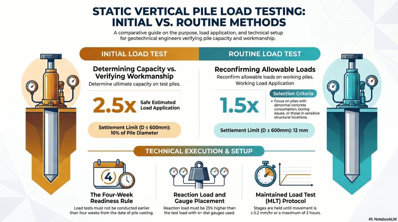
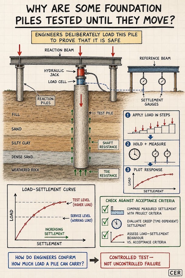
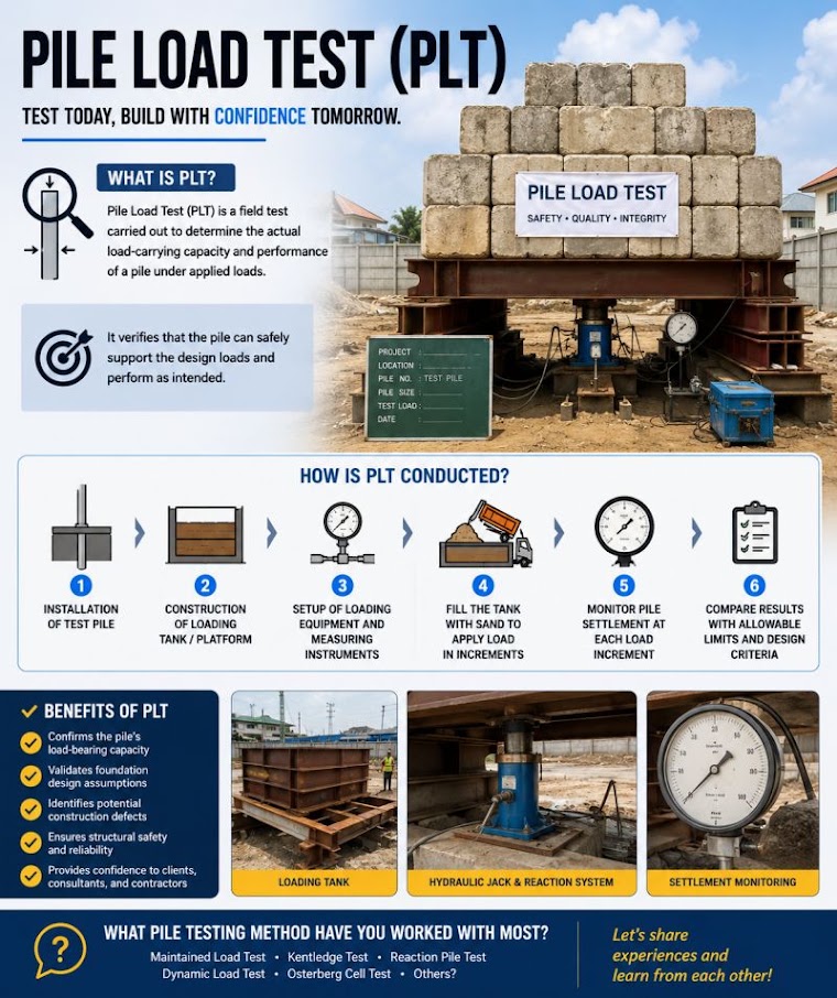
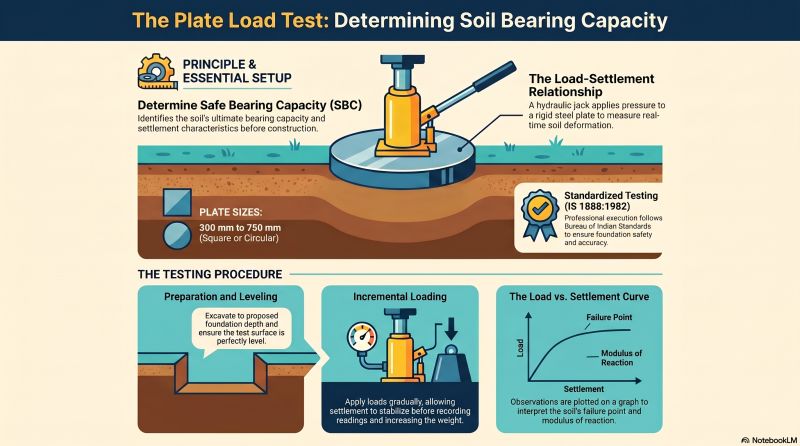
Static load testing is the most reliable method for confirming driven or drilled pile capacity. It is required by UPRR, BNSF, and Amtrak for all new bridge foundations; by CSXT and NSR for projects with design load > 200 tons per pile.
Load is applied in 8% increments of the anticipated failure load, each increment held for 2.5 minutes, until failure or 200% of design load is reached. Total test duration is typically 2–4 hours.
Load application:
Test load applied by hydraulic jack against a reaction system (kentledge deadweight, reaction piles, or helical anchor reaction frame).
Jack force:
P_jack = p_hydraulic × A_ram (lb)
where p_hydraulic = hydraulic pressure (psi) and A_ram = ram area (in.²).
Settlement measurement: Four dial gauges or LVDTs at 90° spacing, referenced to a stable reference beam. Resolution ≥ 0.001 in.
Reference graphics
Reference graphics · click to zoom
Davisson Offset Method (standard for driven piles, adopted by UPRR, BNSF, CSXT, NSR):
Δ_failure = (Q × L) / (A_pile × E_pile) + (D/120) + 0.15 in.
where:
Plot load-settlement curve; intersection of load-settlement curve with Davisson offset line defines Q_failure (tons).
Design capacity: Q_allow = Q_failure / FS
FS = 2.0 (with PDA + CAPWAP); FS = 2.5 (without load test); FS = 2.0 (with static load test) — per AREMA MRE Chapter 8 and UPRR/BNSF Engineering Instructions.
Reference graphics
For UPRR crane rail foundations and BNSF intermodal structure piers, Osterberg Cell (O-Cell) testing is preferred over top-down testing when reaction frames would conflict with existing structures. The O-Cell is a bidirectional load cell embedded in the shaft; it loads the tip against the side in two directions simultaneously.
O-Cell net upward force:
Q_side = Q_cell − Q_tip(mobilized) (lb)
The O-Cell test produces separate side friction and tip resistance load-settlement curves, which are combined analytically to produce the equivalent top-down capacity.
Reference graphics
Reference graphics · click to zoom
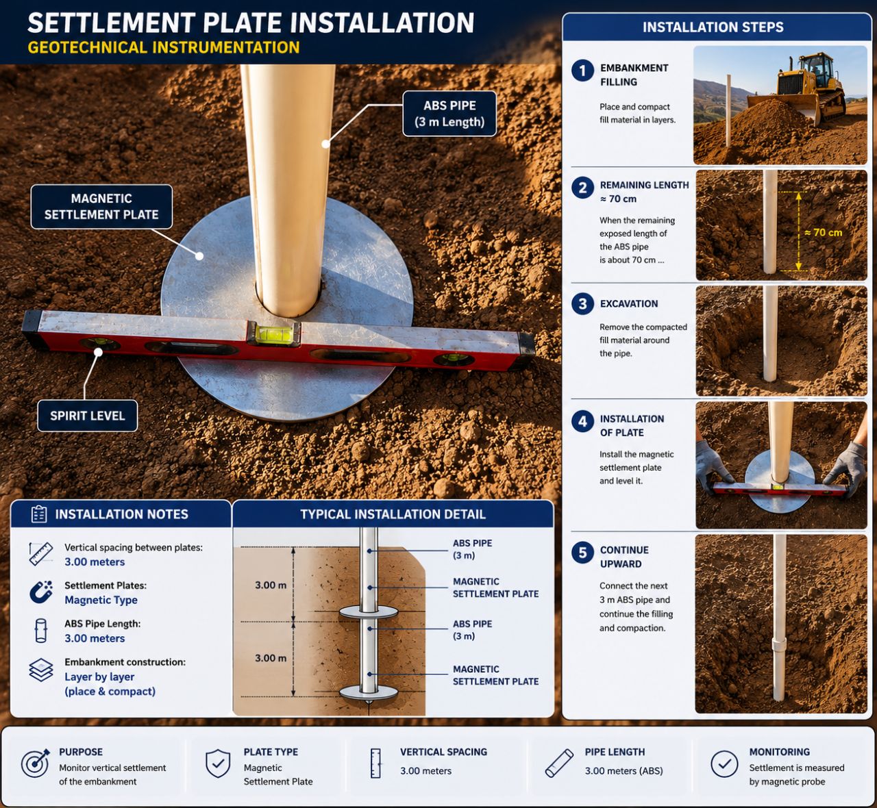
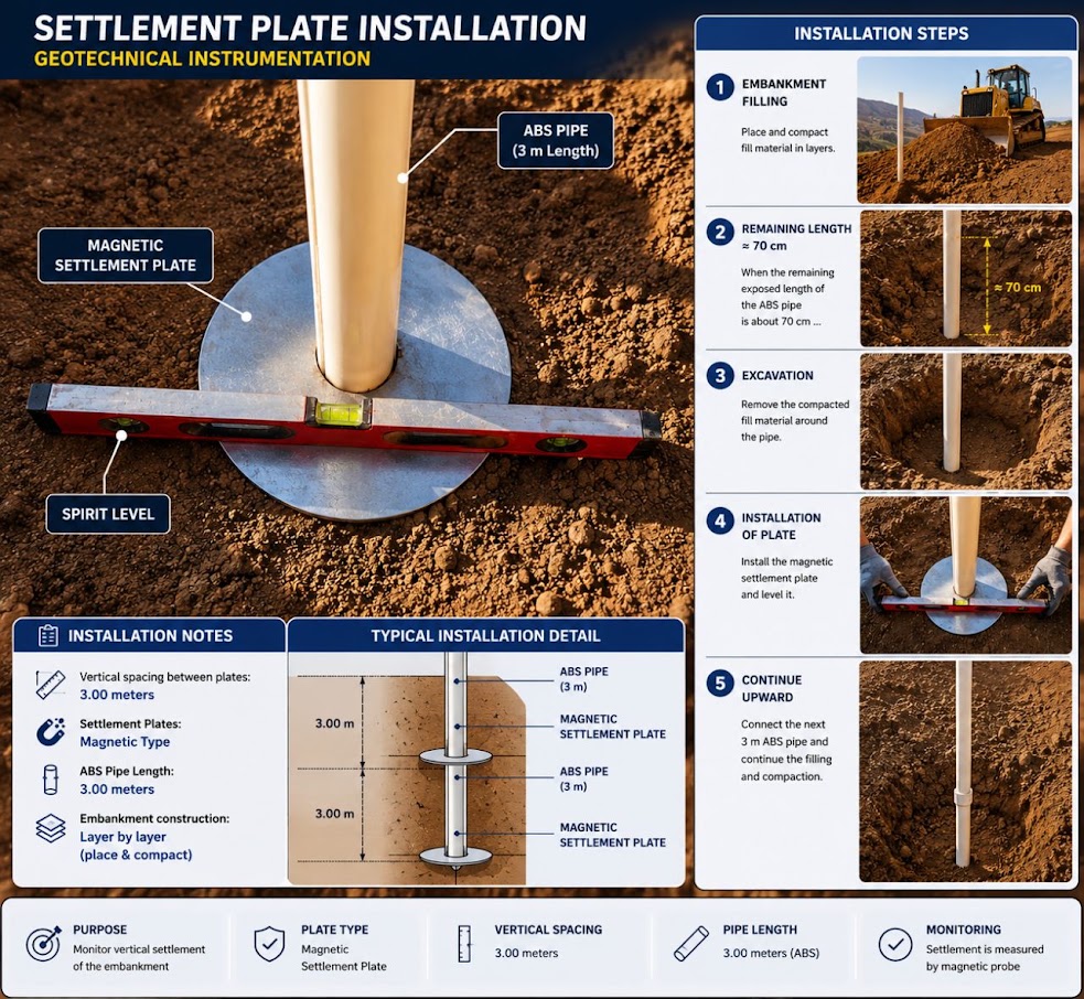
Settlement plates are installed at the base of embankment construction to measure total settlement of the underlying foundation soils during and after filling. They consist of a steel plate (24 in. × 24 in. × ¼ in.) with a vertical measurement rod extending through the embankment fill.
Settlement measurement:
S = E_initial − E_reading (in. or ft)
where E_initial = initial elevation of plate top (ft); E_reading = current survey elevation (ft).
Settlement plates are read by differential leveling survey with ±0.01 ft precision. Reading frequency:
| Stage | Reading Frequency | Purpose |
|---|---|---|
| Embankment filling (active) | Daily or each fill lift | Track rate of settlement vs. fill height |
| End of filling | Daily for first 2 weeks | Confirm no sudden increase |
| Consolidation monitoring | Weekly for first 3 months | Confirm consolidation progressing per design |
| Long-term monitoring | Monthly until ΔS < 0.01 ft/month | Confirm primary consolidation complete |
CSXT Engineering Standards require settlement plate data to be delivered to the project engineer within 24 hours of each reading during active filling.
During staged construction over soft ground (Chapter 17), the fill rate must be controlled to prevent undrained shear failure. The maximum safe fill rate:
ΔH_max per lift = (ΔS_u / γ_fill) × FS_slope (ft/lift)
where:
Field monitoring trigger: if settlement rate increases disproportionately to fill rate (creep rupture indicator), suspend filling immediately and notify the geotechnical engineer. BNSF Engineering Instructions define this as ΔS > 1 in./day without new fill added.
Wayside monitoring of fouled ballast (FRA/BNSF waiver research). Under an FRA waiver from 49 CFR §213.103 (2017–2019, 340 route miles of BNSF track), six solar-powered wayside sites near Lincoln, NE and Kansas City, MO recorded rail and tie strain, accelerations, video displacement and ballast moisture from 2017 to 2020. Support was measured by the distribution efficiency DE = PDist/PC × 100%, where PC is the wheel load from crib strain gauges and PDist is the load still carried by the rail over the tie. DE = 100% is a hanging tie, and a well-supported tie carries about 40% (DE ≈ 40%). Findings:
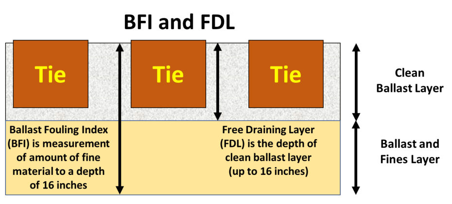
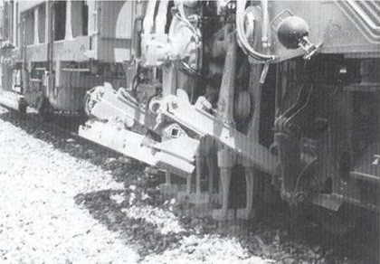
Network GPR (BNSF). BNSF has used ground-penetrating radar since 2009 and in 2018 added it to its train-based geometry car (Figure 15-S1). It reports a Ballast Fouling Index (BFI, the GPR estimate of Selig’s FI = P4 + P200 in the top 16 in.) for the center and shoulders, and since 2018 a Free Draining Layer depth (FDL, 0–16 in. of clean ballast above the fouled zone; Figure 15-S2). Calibration used an automated “Vibro Sampler” for physical gradations. The goal is to group track reliably into clean, moderate and fouled rather than to match FI exactly. BFI and FDL, with geometry, tonnage and maintenance history, feed a model that chooses among surfacing, shoulder ballast cleaning (fast, but does not fix high center fouling), track lifting and undercutting (productivity drops with high fines and moisture), and ditching. For geotechnical work, low FDL with clay-type fines points to a subgrade source, which ballast cleaning alone will not cure.
Source: Stark, T. D., Thompson, H. B., Sussmann, T. R., Bruzek, R. and Banister, R. (2021). “Long-Term Field Monitoring of Fouled Ballast.” AREMA 2021 Annual Conference · Bankston, A. (BNSF) and Wilk, S. (TTCI) (2021). “Use of Track Based Inspection Technologies to Improve BNSF’s Ballast Maintenance Planning.” AREMA 2021 Annual Conference
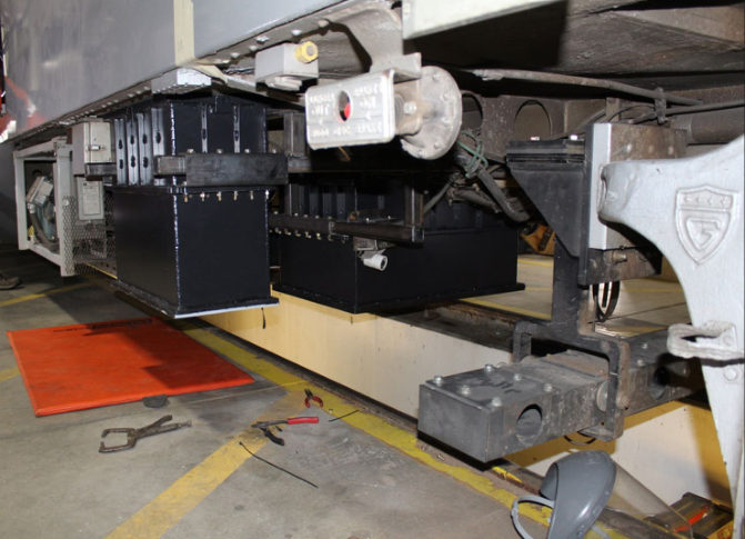
After tamping, a survey crew sets the lift and line corrections, the tamper corrects and compacts under the ties, and a recording car checks the remaining defects against acceptance values. Stabilizing machines that follow the tamper raise lateral resistance. If heavy machinery does the leveling, no further lifts should be made until traffic has stabilized the track. Defects left after that period are corrected with light equipment without re-lifting.
| Track speed (mph) | > 155 | 124–155 | 75–124 | > 50 | < 50 |
|---|---|---|---|---|---|
| Longitudinal defect (in.) | 0.079 | 0.12 | 0.12 | 0.16 | 0.2 |
| Horizontal defect (in.) | 0.079 | 0.12 | 0.12 | 0.16 | 0.2 |
| Track twist (in./ft) | 0.012 | 0.012 | 0.012 | 0.018 | 0.018 |
| Track gauge (in.) | ±0.079 | ±0.079 | ±0.079 | ±0.12 | ±0.12 |
The period up to about 2 million tons after the work (about 1–4 months on a UIC group 4 line, 15–40 days on busier lines) is when defects grow fastest. Profillidis calls continuous monitoring and prompt local correction during this period the key to track longevity. The same window applies after subgrade repairs, undercutting and new embankment tie-ins.
Figures · click to zoom
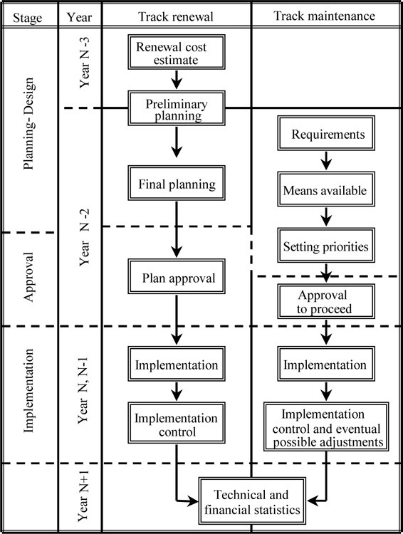
After Profillidis (2014), §16.6.3, §16.8–16.10, Table 16.3, Figs. 16.9, 16.12. Full reference under Supplemental Sources.
During staged embankment filling over soft saturated fine-grained soils, piezometers are installed to monitor excess pore pressure buildup. Rapid excess pore pressure buildup indicates faster loading than the soil can drain, creating instability risk.
Excess pore pressure ratio:
r_u = Δu / σ_v
where Δu = excess pore pressure (psf) and σ_v = total vertical stress increase from fill (psf).
Safe fill criterion: If r_u > 0.5, suspend filling. This is the practical trigger used by CSXT, NSR, and CN for staged construction projects, based on USACE EM 1110-2-1901.
Degree of consolidation from piezometer:
U_field = 1 − (Δu / Δu₀)
where Δu₀ = initial excess pore pressure immediately after fill placement; Δu = current excess pore pressure.
Compare U_field to the design U from the time-rate analysis (Chapter 12). If U_field is lagging behind design U, fill placement may be advanced at a reduced rate; never faster than design.
VW piezometers output a frequency reading (Hz) that is converted to pressure:
P = G × (R − R₀) + K × (T − T₀) (psf or psi)
where:
Typical VW reading cycle: automated datalogger at 15-minute intervals during active filling; hourly during consolidation monitoring. CSXT and Amtrak require automated datalogger downloads every 24 hours to project engineer during active construction.
Reference graphics
Inclinometers measure lateral ground movement (horizontal deflection) in embankments, slopes, and retaining walls. A probe is lowered through a casing installed in a near-vertical borehole to measure deviation from vertical.
Reference graphics
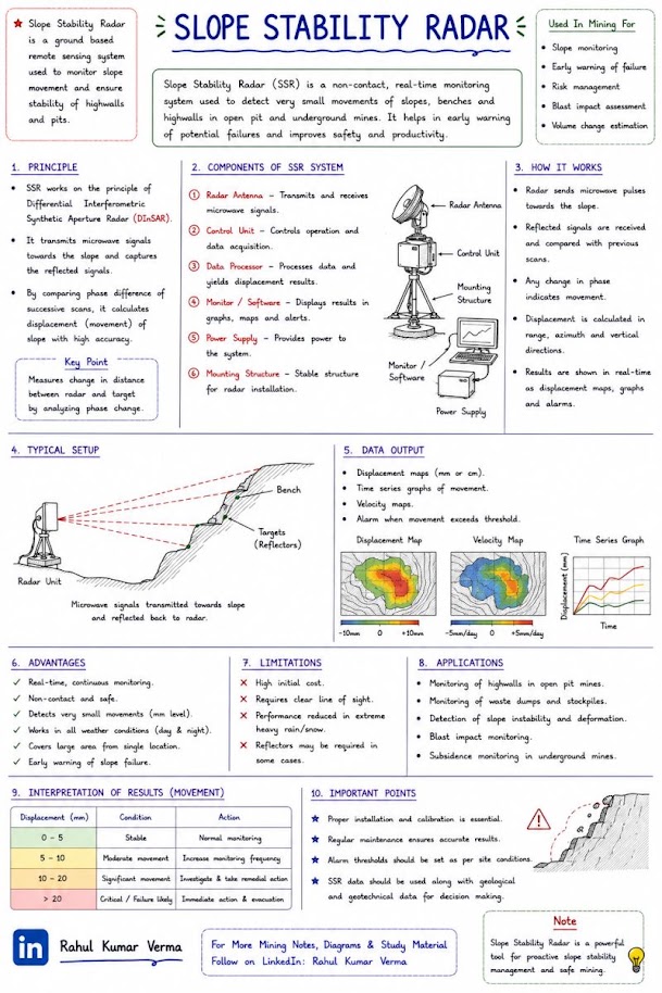
Incremental displacement:
δ_h = L × sin(θ) (in. per segment)
where L = probe wheel spacing (usually 2.0 ft) and θ = tilt angle read by accelerometer (radians or degrees).
Cumulative deflection from depth z to surface:
Δ_H = Σ (L × sin θ_i) (in.)
Plotted as deflection profile vs. depth. The shear zone (zone of maximum rate-of-change of deflection with depth) indicates the failure plane location.
| Trigger Level | Criteria | Action Required |
|---|---|---|
| Alert | Δ_H > 0.25 in. in any 7-day period | Notify geotechnical engineer; increase reading frequency to daily |
| Action | Δ_H > 0.50 in. in any 7-day period | Suspend construction operations in affected zone; convene engineer review |
| Emergency | Δ_H > 0.10 in./day on 3 consecutive days | Immediately halt all loading; implement emergency support if needed; notify RR dispatcher |
Source: Compiled from CSXT Eng. Std., NSR Eng. Std. Manual, UPRR Eng. Instr. Manual, and USACE EM practice.
Reading frequency during active construction:
Before or alongside instruments, crews monitor tension cracks with survey markers driven at the crack and paint marks across it, recording whether it is widening. After stabilization, the course’s program confirms effectiveness through follow-up geotechnical inspections over at least two years, tracked against track-inspection results. Keep records of trench-drain locations, since silt can clog them within 2–6 years.
Figures · click to zoom
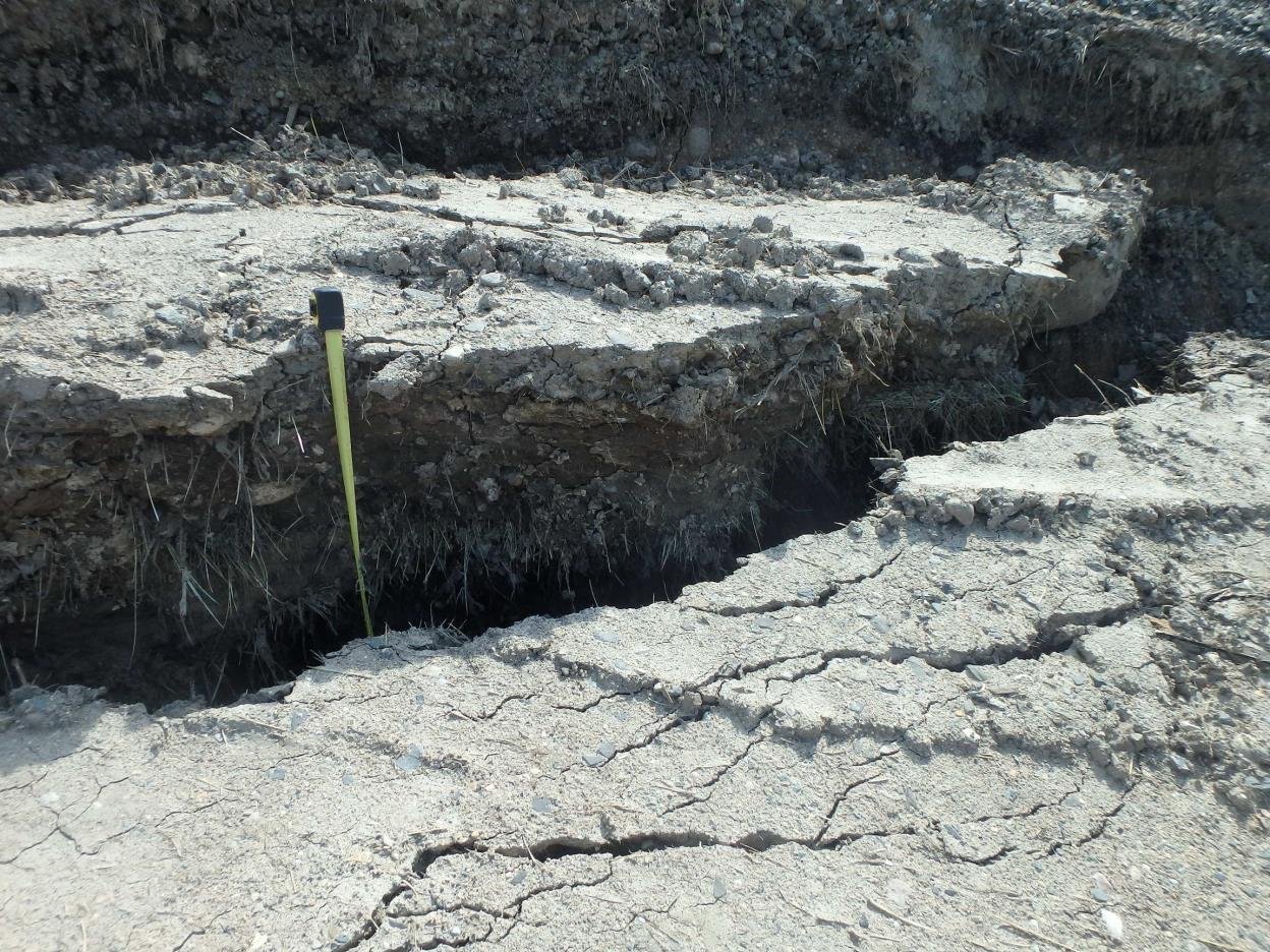
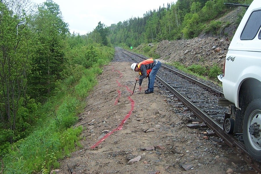
After Geotechnology for Railroaders Program, Module 6.1, Module 7.1, Module 1, Module 6.6; Module 6.1 §05; Module 7.1 §05; Module 1 §10. Full reference under Supplemental Sources.
| Railroad | Compaction Test (method) | Proof Roll (required?) | PDA Piles (%) | Static Load Test | Settlement Plate | Inclinometer | Piezometer | Governing Std. |
|---|---|---|---|---|---|---|---|---|
| CSXT | D6938 nuclear | Yes (mainline) | 5% | > 200T design | Required: staged const. | Soft subgrade | Staged const. | CSXT Eng. Std. Sec. 7 |
| NSR | D6938 or D1556 | Yes (mainline) | 5% | > 200T design | Required: staged const. | Soft subgrade | Staged const. | NSR Eng. Std. Sec. 7 |
| G&W | D6938 or D1556 | Case-by-case | Not required | Not required | Case-by-case | Case-by-case | Case-by-case | G&W Eng. Bulletin |
| UPRR | D6938 nuclear | Yes (mainline) | 10% | All bridges | Required: staged const. | Staged const. | Staged const. | UPRR Eng. Instr. Manual |
| BNSF | D6938 nuclear | Yes (mainline) | 10% | All bridges | Required: staged const. | Staged const. | Staged const. | BNSF Eng. Instructions |
| CPKC | D6938 nuclear | Yes (mainline) | 10% | All bridges | Required: staged const. | Staged const. | Staged const. | CPKC Track Standards |
| Amtrak | D6938 or D1556 | Yes (all track) | 100% (NEC) | All bridges | Required: all | All embankments | All soft ground | Amtrak Eng. Std. |
| CN | D6938 nuclear | Yes (mainline) | 10% | All bridges | Required: staged const. | Staged const. | Staged const. | CN Eng. Standards |
Reference graphics

Reference graphics · click to zoom
The geotechnical inspector is responsible for a daily field report for each day of active monitoring. Minimum content:
All nine client railroads require daily field reports to be submitted electronically (PDF) within 24 hours. CSXT uses ProjectWise; UPRR and BNSF use their proprietary project management portals; NSR requires submission to the project engineer of record by email with a structured naming convention.
Reference graphics
| Test No. | Date | Station | Lift No. | Depth (in.) | γ_d,field (pcf) | MC (%) | γ_d,max (pcf) | RC (%) | Min. RC (%) | Pass/Fail |
|---|---|---|---|---|---|---|---|---|---|---|
| 001 | 06/01/26 | 240+50 | 3 | 6 | 121.4 | 10.2 | 127.0 | 95.6 | 95.0 | Pass |
| 002 | 06/01/26 | 241+00 | 3 | 6 | 118.7 | 12.5 | 127.0 | 93.5 | 95.0 | Fail |
| 003 | 06/01/26 | 241+00 | 3 | 6 | 122.1 | 10.8 | 127.0 | 96.1 | 95.0 | Pass (retest) |
A pile driving log must be completed for every driven pile:
UPRR and BNSF Engineering Instructions require the final pile driving log to be signed by both the geotechnical inspector and the railroad construction inspector.
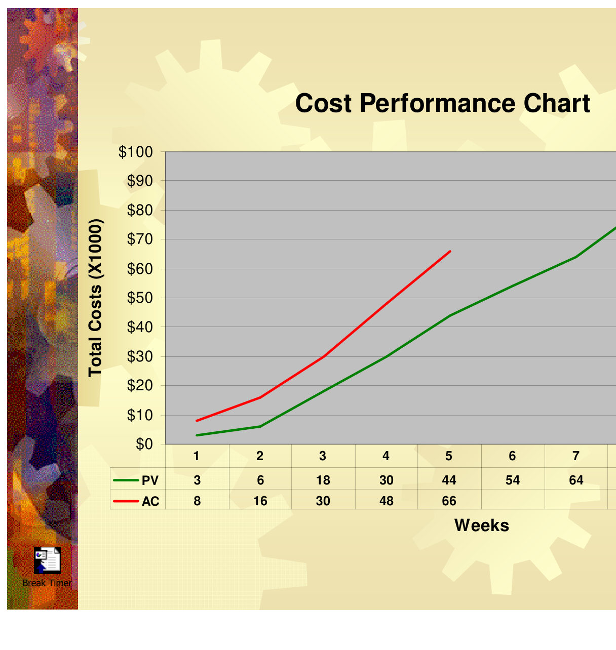
During execution, the course compares progress to plan with three tools: quality reviews, Gantt schedule performance charts and cost performance charts. Its cost chart plots cumulative planned value (PV) against cumulative actual cost (AC) by week. In the example, planned value reaches $44,000 by week 5 against an actual cost of $66,000, so spending is 50% above plan and the gap has widened every week.
Table 15-PM1. Cumulative planned value and actual cost, $1,000 (after Skill Right 2013, Cost Performance Chart)
| Week | 1 | 2 | 3 | 4 | 5 |
|---|---|---|---|---|---|
| PV | 3 | 6 | 18 | 30 | 44 |
| AC | 8 | 16 | 30 | 48 | 66 |
For change, the course separates customer-requested changes (usually the largest source) from internal requests, regulation and team-generated changes. Its procedure is: hold a team meeting, explain the change, get feedback, identify alternatives, prepare a decision matrix, select a recommendation, present it to management or the customer, and implement the approved course.
For railroad work: a PV-versus-AC chart cannot by itself tell overspending apart from work being done ahead of schedule. Add the budgeted value of the work actually performed, measured in physical units: inspector shifts actually needed, density tests, piles observed, monitoring rounds and reports issued. Construction-phase geotechnical budgets on railroad projects are often consumed by standby and repeat mobilizations when track windows are cancelled or the contractor’s sequence changes. Log those days as a separate cost line from the first occurrence. Then, when the change procedure is invoked, the decision matrix compares real alternatives:
Report cost status with the same frequency and in the same document as the QA/QC test summaries, so the railroad sees quality, schedule and cost together.
Source: Skill Right (2013). Project Management Tools and Techniques: An Introductory Course in Project Management Foundations [training slides sponsored by Texas Instruments, Inc.; minor modifications by N. Santiago, Spring 2013 version], slides 81–83, 86–87. Summarized and paraphrased; figures reproduced for internal reference. Full reference under Supplemental Sources.
Sears et al. list the main sources of project change: added or altered work ordered by the owner or engineer, contractor value-engineering proposals, delays caused by the owner or other contractors, and job-site conditions that differ materially from those anticipated. Their procedure for handling a change:
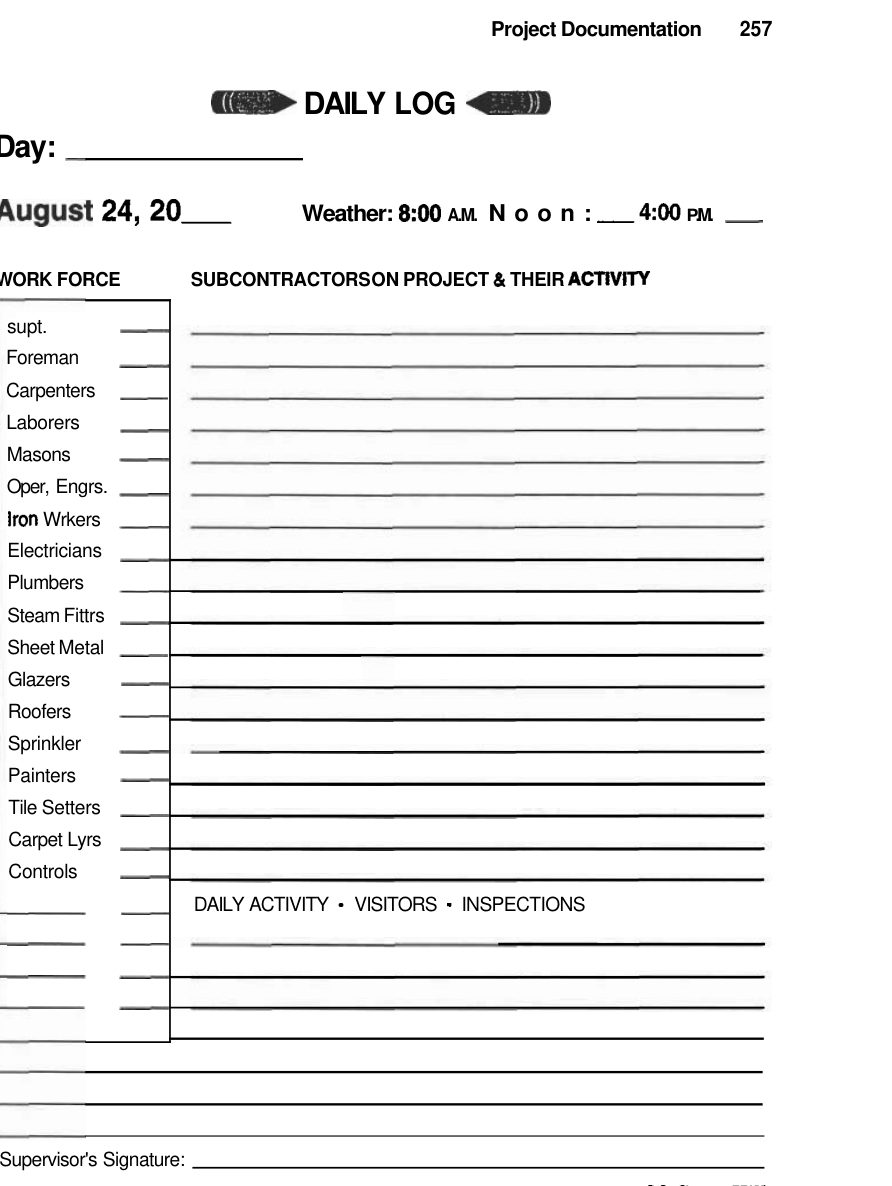
Their rule for claims is documentation, and the core record is the daily job log. Each entry records the date, weather, workers by craft, equipment by type, activities started and finished with quantities, subcontractors on site, deliveries (including late or damaged ones), visitors and inspectors, meetings and decisions, problems, and corrective steps. To be accepted as evidence, entries must be original, made on the date shown in the regular course of business, based on the writer’s own knowledge, and kept in a bound book or an equivalently secure electronic system. Entries should state facts without opinion or emotion.
For railroad work: The inspector’s daily report on a railroad job should add the items that drive most disputes there: the track window granted versus planned, with start and stop times; flagging availability; train delays and slow orders in effect; and quantities of undercut, unsuitable material removed and fill placed by station. When the subgrade exposed in an undercut differs from the boring logs, photograph it, note the stations and depths, and notify the railroad’s representative the same day. Then run the “with and without change” schedule comparison before the next window is booked.
Source: Sears, S. K., Sears, G. A., Clough, R. H., Rounds, J. L., and Segner, R. O., Jr. (2015). Construction Project Management: A Practical Guide to Field Construction Management, 6th ed. Hoboken, NJ: John Wiley & Sons, pp. 328–332. Summarized and paraphrased. Full reference under Supplemental Sources.
Levy (2007) treats documentation as part of the work itself and places his documentation chapter immediately before the one on claims for that reason. Good records are not volume; they are prompt, accurate entries made when important events happen. For any significant event he recommends recording what happened, when and how it happened, when it was discovered, whether responsibility can be assigned with certainty, who was notified and when, its impact, the immediate and longer-term actions required and by whom, and which party will resolve it. Facts should be separated from opinions; useful remarks at meetings can be noted separately to show intent.
The superintendent’s daily record is the backbone. Levy notes that a bound diary with daily entries meets the legal definition of a business record, while loose sheets may not, and suggests reviewing electronic logs with counsel. At a minimum each entry should give the date (with “No Work” on idle days); weather and temperature at start, midday and end of shift; each subcontractor on site with crew size, work and location; the firm’s own workforce and tasks; visitors and their purpose; inspections by agencies, testing labs or the engineer; work performed and where; deliveries with ticket numbers; unusual events and stoppages; and every accident, reportable or not.
Photographs document progress or lack of it, conditions that differ materially from those expected, support for change orders, and complex details. Levy recommends a tape or rule in close-ups for scale, and specifically lists rock, groundwater and buried debris as conditions to photograph even when they seem unlikely to matter contractually. His closing advice is simply: document, document, document.
For railroad work: The geotechnical field representative’s daily report on a subgrade rehabilitation, slide repair or culvert replacement should add railroad-specific fields: track and work-window times granted and released, the employee in charge or flagman, trains passed during the window, any slow order in effect, and lost window time with its cause. Photograph undercut subgrade, seepage, slip surfaces and unsuitable material in place with a scale and a station reference before it is removed or covered, and link each photo to the daily report and test locations.
Source: Levy, S. M. (2007). Project Management in Construction, 5th ed. New York: McGraw-Hill, pp. 229–230, 255–260. Summarized and paraphrased; figures reproduced for internal reference. Full reference under Supplemental Sources.
Goldbloom states a basic rule: responsibility for the result follows whoever prescribed the method. If a specification dictates how the work is done and the contractor follows it, the contractor is not liable for a bad result. His common bad example is embankment specifications that fix loose-lift thickness, compactor type and size, and number of passes, and then also demand a minimum in-place density. When the procedure is followed and the density is missed, the owner has no position. His recommended end-result approach is to:
Lift thickness, moisture, the dumping method, and the type and size of the compactor all affect the number of passes needed. That is why the means should be left to the contractor.
He also separates two functions:
Each technical section should say which tests the engineer will perform and by what method, so the contractor knows how acceptance will be judged. His cautionary example is a contract that made the contractor hire the testing laboratory for in-place density, batch-plant inspection and concrete cylinders. A lab paid by the contractor owes its first loyalty to the contractor, so this cannot serve as QA.
On tolerances, he notes that rigid wording such as “true to line and grade” leads to claims. In one spillway case the court allowed the contractor to recover the cost of forming to tolerances tighter than the finished structure required.
For railroad work: Ballast, subballast and subgrade QA/QC documentation should state for each item whether it is an end-result or a method requirement, and should not mix the two. When a method requirement is unavoidable, such as track-time-limited proof rolling or prescribed lift placement under a work window, write the acceptance criterion as conformance to that method. Keep acceptance testing (nuclear gauge, plate load, proof roll observation) with the railroad’s representative or its own consultant. Contractor testing should be identified as QC only. Give grade and cross-slope tolerances that track and drainage design can actually live with.
Source: Goldbloom, J. (1989). Engineering Construction Specifications: The Road to Better Quality, Lower Cost, Reduced Litigation. New York: Van Nostrand Reinhold, pp. 20–21, 183–184, 188. Summarized and paraphrased. Full reference under Supplemental Sources.
Anglin works through the general-conditions clause on concealed or unforeseen conditions, quoting AIA A201 (Article 4.3.4), and illustrates it with a case from his own practice. The clause recognizes two types:
Whoever observes the condition must give notice promptly, before it is disturbed, and in any case within 21 days. The architect or engineer then investigates. If the condition does differ materially, a change follows; if not, the reasons must be given in writing. Anglin stresses giving written notice of cost or delay even before the amount is known. A continuing delay needs to be documented only once.
In his fire-college case, excavation for a new building uncovered a fire line that turned unexpectedly under the footprint. The contractor took these steps:
The owner argued that a plan note required the contractor to field-verify utilities. The contractor answered that, under the contract, studying the documents is meant to facilitate construction, not to discover errors. He also showed that no one had specified a particular sequence of excavation. The owner paid.
For railroad work: on subgrade, slope and culvert jobs, the geotechnical field representative is usually the first to see the condition. Typical examples are:
The daily report should record:
Railroad and agency contracts set their own notice periods and procedures, so put them in the field instructions before work starts.
Source: Anglin, G. (2020). Introduction to Estimating, Plan Reading and Construction Techniques. Abingdon: Routledge, pp. 381–382, 387–390. Summarized and paraphrased. Full reference under Supplemental Sources.
Project context: CSXT Georgia Division bridge abutment replacement. Structural fill compacted with a Cat 836K landfill compactor. Modified Proctor reference: γ_d,max = 125.5 pcf at w_opt = 11.2%.
Given (nuclear gauge readings from Test 014):
Step 1: Field dry density
γ_d,field = WD / (1 + MC/100) = 139.4 / (1 + 0.118) = 139.4 / 1.118 = 124.7 pcf
Step 2: Relative compaction
RC = (124.7 / 125.5) × 100% = 99.4%
Step 3: Compare to specification
CSXT requirement for structural fill: RC ≥ 95%. RC = 99.4% >> 95% ✓
Step 4: Moisture check
CSXT Engineering Standards require moisture within ±3% of w_opt = 11.2%: acceptable range 8.2%–14.2%. Field MC = 11.8% ✓
Result: Test 014 — PASS. Document on daily field report and compaction test log.
Project context: UPRR Columbia River crossing. 14-in. H-pile (HP14×117), L = 75 ft, driven with ICE 660 hydraulic hammer (E_rated = 66,000 ft·lb). PDA equipped. Clay subgrade.
Given (PDA record at final set):
Step 1: Pile impedance
Z = (29 × 10⁶ psi × 144 in.²/ft² × 34.4 in.²) / (16,808 ft/s × 144)
Actually: Z = (E × A) / c with consistent units:
E = 29 × 10⁶ lb/in.² × 144 in.²/ft² = 4.176 × 10⁹ lb/ft²
Z = (4.176 × 10⁹ × 34.4/144) / 16,808 = (4.176 × 10⁹ × 0.2389) / 16,808 = (997,646,400) / 16,808 = 59,356 lb/(ft/s) ≈ 59,400 lb·s/ft
Step 2: Case Method capacity
R_total = ½ × (1 + 0.50) × [650,000 + 59,400 × 8.5] + ½ × (1 − 0.50) × [280,000 + 59,400 × (−2.1)]
= ½ × 1.50 × [650,000 + 504,900] + ½ × 0.50 × [280,000 − 124,740]
= 0.75 × 1,154,900 + 0.25 × 155,260
= 866,175 + 38,815 = 905,000 lb = 452 tons
Step 3: Allowable capacity
Q_allow = 452 / 2.0 (FS with PDA + CAPWAP restrike) = 226 tons
Design load = 180 tons. FS_actual = 452 / (180 × 2) = 1.26... Wait — with PDA: Q_allow = R_total / FS = 452 / 2.0 = 226 tons > 180 tons design ✓
Conclusion: Pile meets design load requirement. Schedule CAPWAP analysis of this record and two additional PDA records per UPRR requirements.
Project context: NSR Alabama Division embankment over soft Gulf Coast clay. Staged construction with PVDs installed. Current embankment height H = 12 ft (fill placed in last 3 days). VW piezometer at 15 ft depth reads Δu = 850 psf. Fill unit weight γ_fill = 122 pcf.
Step 1: Vertical stress increase from new fill
σ_v = γ_fill × H = 122 × 12 = 1,464 psf
Step 2: Excess pore pressure ratio
r_u = Δu / σ_v = 850 / 1,464 = 0.581
r_u = 0.581 > 0.50 → Action threshold exceeded.
Step 3: Required response
Per NSR Engineering Standards and USACE EM 1110-2-1901: suspend filling immediately. Notify NSR project engineer and geotechnical engineer within 1 hour. Increase piezometer reading frequency to every 2 hours. Do not resume filling until r_u falls below 0.35 (NSR staged construction protocol).
Step 4: Field consolidation check
Settlement plate data shows ΔS = 0.82 in. over last 3 days (0.27 in./day). No excessive rate yet but r_u exceeded. This is consistent with rapid load application exceeding drainage capacity of PVDs. Verify PVD installation spacing matches design (see Chapter 17).
Step 5: Document
Issue written Piezometer Alert notification to NSR project manager, contractor superintendent, and NSR construction inspector within 24 hours (NSR Engineering Standards requirement). Attach VW reading log and r_u calculation.
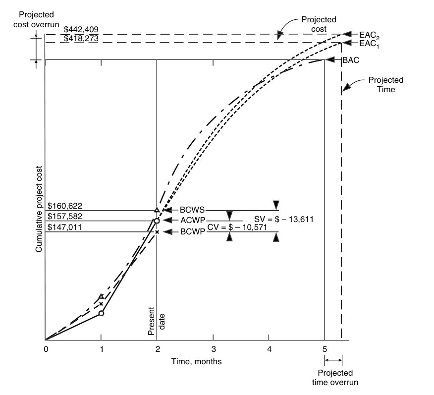
Sears et al. point out that a standard monthly cost forecast shows only whether the job will finish over or under budget. It cannot tell whether the variance comes from cost performance, schedule performance or both. The earned value management system (EVMS) separates the two by comparing three cumulative quantities at each update:
From these: cost variance CV = BCWP − ACWP; schedule variance SV = BCWP − BCWS, expressed in dollars; CPI = BCWP/ACWP; SPI = BCWP/BCWS. An index below 1.0 calls for management attention. The estimate at completion is bracketed by EAC1 = ACWP + (BAC − BCWP)/CPI and EAC2 = ACWP + (BAC − BCWP)/(CPI × SPI), where BAC is the budget at completion. The to-complete index TCPI = (BAC − BCWP)/(EAC − ACWP) gives the cost efficiency needed on the remaining work.
Source example (highway bridge, day 27): BAC = $390,214; BCWS = $160,622; BCWP = $147,011; ACWP = $157,582. Then CV = −$10,571 and SV = −$13,611; CPI ≈ 0.93 and SPI ≈ 0.92. The forecast range is EAC1 ≈ $418,273 to EAC2 ≈ $442,409. In other words, if the cost inefficiency continues, the job finishes about $28,000 over, and continued schedule slippage could raise that to about $52,000.
The authors also describe the time-cost envelope (early-start and late-start cumulative cost curves) as the graphical forerunner of EVMS.
For railroad work: On a unit-price subgrade rehabilitation or slope repair, use the bid items as the budget lines and the construction monitoring quantities (cubic yards of undercut, tons of subballast or riprap, linear feet of drain, piles driven) as the earned value. Because work is confined to track windows, a low SPI often means windows were lost or shortened, not that crews were slow. Keep the window log next to the EV report so the cause is clear. A falling CPI combined with deeper-than-planned undercut is an early quantitative sign of a differing-condition trend that should be raised with the railroad before the next window, not at close-out.
Source: Sears, S. K., Sears, G. A., Clough, R. H., Rounds, J. L., and Segner, R. O., Jr. (2015). Construction Project Management: A Practical Guide to Field Construction Management, 6th ed. Hoboken, NJ: John Wiley & Sons, pp. 298–303. Summarized and paraphrased; figures reproduced for internal reference. Full reference under Supplemental Sources.
| Day | Fill H (ft) | σ_v (psf) | Δu (psf) | r_u | S_plate (in.) | ΔS/day (in.) | Status |
|---|---|---|---|---|---|---|---|
| 0 | 0 | 0 | 0 | 0 | 0 | — | Baseline |
| 3 | 4.0 | 488 | 195 | 0.40 | 0.22 | 0.07 | OK |
| 7 | 8.0 | 976 | 440 | 0.45 | 0.68 | 0.11 | OK |
| 10 | 12.0 | 1,464 | 850 | 0.58 | 1.50 | 0.27 | Alert — Suspend |
| 14 | 12.0 | 1,464 | 610 | 0.42 | 2.10 | 0.15 | Consolidating |
| 21 | 12.0 | 1,464 | 385 | 0.26 | 3.20 | 0.16 | OK — Resume fill |
| 25 | 15.0 | 1,830 | 520 | 0.28 | 3.85 | 0.16 | OK |
| 35 | 18.0 | 2,196 | 490 | 0.22 | 5.10 | 0.13 | OK |
Reference graphics
Reference graphics
Reference graphics · click to zoom
Inherent quality is set at construction. After every tamping, track drifts back toward the shape it acquired when it was built or renewed. Three findings show how strong this effect is:
Undercutter depth control. On a manually controlled undercutter, the cut depth follows the machine’s bogies, and deviations of about ±3 in. were recorded. Laser or water-level control gives a far smoother cut. Specify it, together with a cut surface sloped to the side drains that does not damage an existing blanket.
After tamping. Tamping loosens the cribs and shoulders, so lateral resistance drops. It is substantially regained after about a month of traffic.
Tamping policy. Tamp only when geometry requires it. A low-lift tamp does not produce a lasting improvement; a lasting change needs a lift greater than the ballast D50. Stoneblowing complements tamping: use it for low lifts and short-wavelength faults, and use tamping for high lifts and long-wavelength faults.
After Selig & Waters (1994), chs. 14 and 15. Full reference under Supplemental Sources.
Haidar reviews how extensions of time are calculated when an excusable event occurs while the contractor is already late through its own fault (culpable delay). Under the gross method, the extension runs from the date the event occurred, which sets a new completion date and removes liquidated damages up to it. Under the net method, the contractor receives only the time needed to absorb the event, added to the original completion date. In his example, a contractor six months late is delayed one further month by a relevant event. Under the net method the completion date moves one month past the original date, and five months of culpable delay remain exposed to liquidated damages. The net approach follows Lord Denning’s reasoning in Amalgamated Building Contractors v Waltham Holy Cross (1952).
On concurrent delay, Haidar cites Henry Boot v Malmaison (2000). If a week of work is lost both to exceptional weather (an excusable event) and to a labor shortage (not excusable), the contractor may still be entitled to a one-week extension. He warns that retrospective CPM analysis of very large networks is unreliable, because every logic link is an assumption and a network can be adjusted to make almost any work critical. Liquidated damages work only if the contract also provides a workable extension mechanism. To recover for constructive acceleration, a contractor must show that the owner failed to grant an adequate extension, insisted on the original date, received notice that the contractor was treating this as acceleration, and that extra cost was actually incurred. The cases cited are English, so the governing contract and jurisdiction control on any U.S. project.
For railroad work: the geotechnical field record is often the evidence in these analyses, so record in daily reports:
With all four recorded side by side, the railroad and the contractor can separate excusable delay from culpable delay without reconstructing events months later.
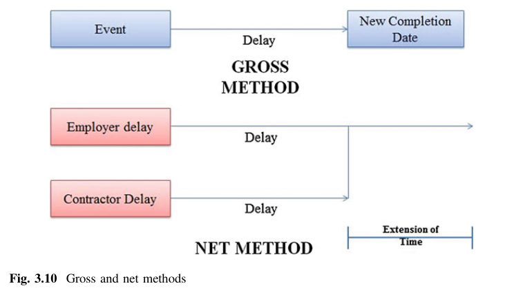
Source: Haidar, A. D. (2016). Construction Program Management – Decision Making and Optimization Techniques. Cham, Switzerland: Springer International Publishing, pp. 75–79. Summarized and paraphrased; figures reproduced for internal reference. Full reference under Supplemental Sources.
Cretu et al. stress that risk management fails most often after the analysis is finished. They invert the usual pyramid: planning and analysis take less effort than carrying out and tracking the responses. Their monitoring and control step includes tracking every risk in a master register, identifying new risks and retiring old ones, adjusting responses that are not working, managing the risk reserve (contingency) as it is spent, and checking that responses are actually carried out. Each risk gets an owner and a task manager who tracks how well the response works and reports on a set schedule. Updates go back to a single master register held by the project manager. The response action plans can be loaded into the project schedule as dated activities so that overdue responses stand out at each status date. On large projects the authors recommend formal risk reviews at the end of concept development (where “project-killer” risks surface), during preliminary design and during final design (construction and contract risks), with interim reviews during construction.
They close with keys to success from NCHRP Report 658. These include: identify risks early and tie contingencies to explicit risks; communicate cost uncertainty as ranges or explicit contingency; assign responsibility for each risk; and monitor threats and opportunities as the way to resolve contingency. They also note that responsibility shared by everyone tends to end up with no one.
For railroad work: Construction monitoring data are the evidence for retiring or escalating geotechnical risks. Link each instrument and test program to the register entries it tests. For example, inclinometer and piezometer readings during staged fill test the “foundation instability” risk, and proof-rolling and density results test the “unsuitable subgrade quantity” risk. Set the threshold that would trigger the planned response. Report contingency drawdown against those same entries at each progress meeting, so the railroad can see that the reserve is being spent on risks that actually occurred or released as they are retired, not absorbed by unrelated changes.
Source: Cretu, O., Stewart, R. and Berends, T. (2011). Risk Management for Design and Construction. Hoboken, NJ: John Wiley & Sons, pp. 149–150, 164–168. Summarized and paraphrased. Full reference under Supplemental Sources.
Checklist · Part VII · Stabilization Methods
Pre-Construction
During Construction
Post-Construction
| Topic | See Also |
|---|---|
| Pile capacity design (static analysis) | Chapter 11 |
| Embankment settlement during construction | Chapter 12 |
| Staged construction slope stability | Chapter 13 |
| PVD design for staged construction | Chapter 17 |
| Subgrade compaction specification | Chapter 18 |
| Retaining wall construction monitoring | Chapter 16 |
| Geotechnical Special Provisions (construction) | Appendix C |
| Final report construction monitoring section | Appendix E |
| Lab testing for reference Proctor | Chapter 10 |
Q1. A nuclear gauge reads WD = 135.8 pcf and MC = 9.5% on a compacted embankment fill. The Modified Proctor reference is γ_d,max = 130.2 pcf. Calculate: (a) γ_d,field, (b) RC, and (c) does this pass UPRR's 92% compaction requirement?
Answer:
Q2. A 12-in. diameter concrete pile (E = 57,000√4,500 psi = 3,824,000 psi; A = 113.1 in.²; L = 60 ft) is tested using ASTM D1143. At Q = 300 kips, total measured settlement is 0.68 in. Calculate the Davisson offset limit and determine if failure has occurred.
Answer: Davisson offset: Δ_failure = (Q × L) / (A × E) + D/120 + 0.15
= (300,000 lb × 60 ft × 12 in./ft) / (113.1 × 3,824,000) + 12/120 + 0.15
= (216,000,000) / (432,754,400) + 0.10 + 0.15
= 0.499 + 0.10 + 0.15 = 0.749 in.
Measured settlement = 0.68 in. < 0.749 in. → Failure has NOT occurred at Q = 300 kips. Continue loading.
Q3. A VW piezometer in a staged construction project reads R = 5,280,000 (Hz²) and R₀ = 5,210,000 (Hz²). Gauge factor G = 0.0015 psi/digit; temperature correction is negligible. New fill added in the last 24 hours: H = 6 ft, γ_fill = 120 pcf. (a) Calculate Δu. (b) Calculate σ_v from the new fill. (c) Calculate r_u. (d) Is filling safe to continue?
Answer:
Q4. An inclinometer casing shows the following cumulative deflections (A-direction, positive toward fill) over three consecutive weekly readings: Week 1: 0.15 in., Week 2: 0.38 in., Week 3: 0.65 in. (a) Calculate the weekly incremental movements. (b) Do any weeks trigger the Action level? (c) What action is required?
Answer:
Q5. A proof roll of prepared subgrade identifies two soft spots at Sta. 185+50 and Sta. 186+20 where rutting exceeds ½ in. Nuclear gauge tests at these locations give RC = 88.2% and RC = 86.5% vs. BNSF's 92% minimum. (a) What is the corrective action? (b) After rework, the re-test gives γ_d,field = 126.8 pcf and γ_d,max = 133.5 pcf. Does this pass?
Answer:
Field case studies by Burt G. Look, from Earthworks: Theory to Practice – Design and Construction (CRC Press/Balkema, 2023), chosen for this chapter’s topics. Each is summarized from the book with its key figures and a closing note on railroad application added by the authors of this manual. Credit for the case material belongs to Look; see item S12 under Supplemental Sources.
Related section: 15.2 Compaction Testing
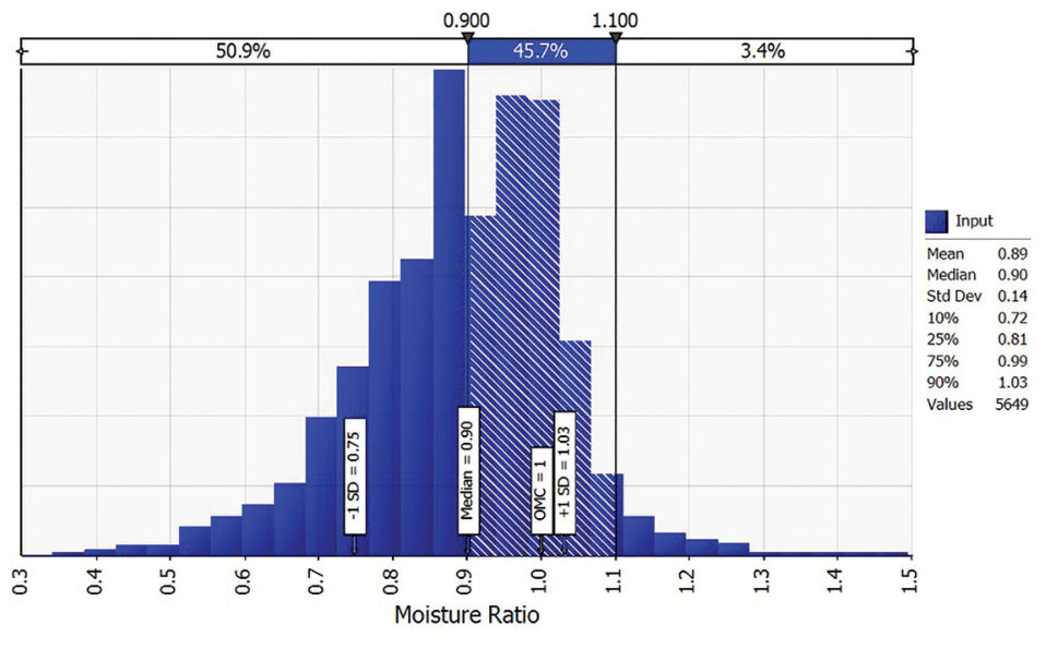
Look examined 5,649 compaction results, mainly low- to medium-plasticity material, all meeting a 95% density ratio target. Placement moisture was mostly dry of optimum:
The median was 90% of OMC, with a ±1 standard deviation range of 75%–103%. Heavy equipment has its own “optimum” dry of laboratory OMC because it delivers so much energy. For 279 tests on high-quality base material (CBR 45), the median density was 103% of MDD at a median moisture of only 63% of OMC.
Laboratory OMC is not a requirement for reaching density in the field. It ignores both the equipment used and the moisture the material will reach in service.
For railroad work: on embankment and subgrade work, a density pass with heavy rollers dry of OMC is common. Where the fill is a plastic clay that will wet up afterwards, see the expansive-clay case under Chapter 3, §3.2.
Source: Look, B. G. (2023). Earthworks: Theory to Practice – Design and Construction. CRC Press/Balkema. Case study §7.8, pp. 228–230. Summarized and paraphrased; figures reproduced for internal reference. Full reference under Supplemental Sources.
Related section: 15.4 Pile Installation Monitoring
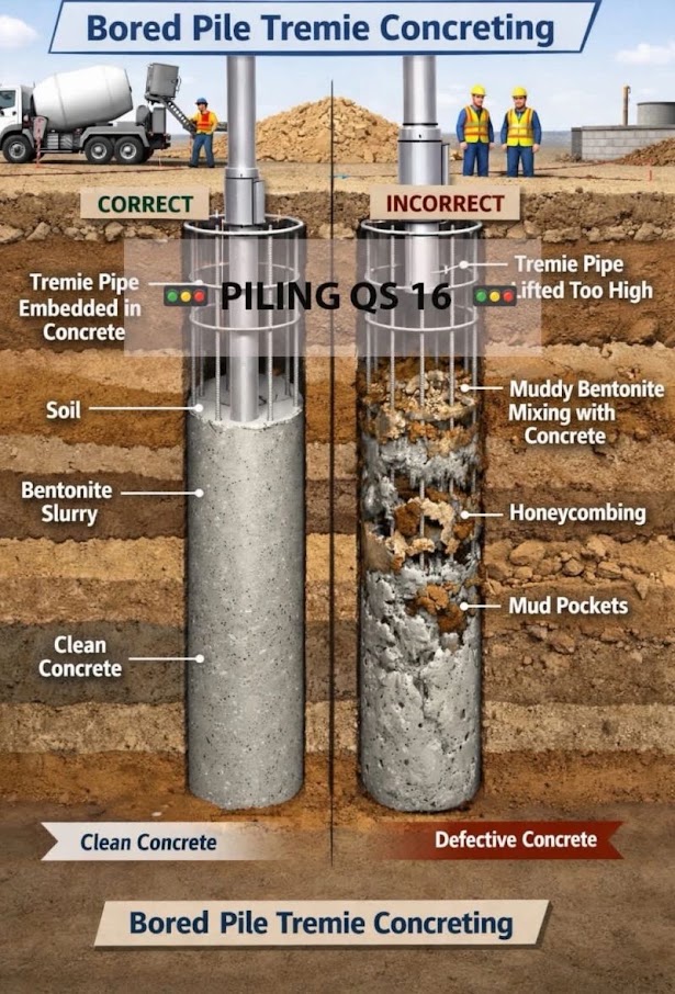
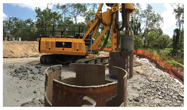
A temporary liner was socketed to the top of rock for a bored pile. While soil was being extracted from inside the liner, a sinkhole opened next to it: bedrock dipped at depth, the liner was embedded unevenly, and material caved in under the edge. The piling rig and the site supervisor were right beside the liner. The operator reversed the rig and the supervisor stepped away in under a minute, and nobody was hurt.
The platform itself was correctly designed; no working platform can bridge a void of this kind. Look draws three points from it: rig operators must be ready to act without notice, so phones should be restricted in critical areas; old trenches and services should be marked and avoided; and instrumentation (survey, inclinometers, extensometers, settlement gauges, piezometers, earth pressure cells) gives early warning, and should be mandatory where the factor of safety is 1.2 or less. Offset distances of about 6.6 ft, or three times the track width of tracked plant, should be kept from any sloping edge.
For railroad work: bridge piling next to live track adds train surcharge and vibration to the same mechanism. Casing embedment on sloping rock should be confirmed, and the exclusion zone around an open casing should be part of the track-protection briefing.
Source: Look, B. G. (2023). Earthworks: Theory to Practice – Design and Construction. CRC Press/Balkema. Case study §3.6, pp. 88–90. Summarized and paraphrased; figures reproduced for internal reference. Full reference under Supplemental Sources.
Authors: Daniel P. Colwell and Mario Ruel. This chapter was written and compiled by Daniel P. Colwell and Mario Ruel for Railway Ground Hazard Risk Management.
Technical content is drawn from the published sources below, and credit for that material belongs to their authors and publishers. Tables, equations and figures taken from a specific source are also cited where they appear.
File locations for these documents are listed under Supplemental Sources — LEVI Library.
Material in the green “Supplemental reference” boxes throughout this chapter was added from the following documents in the LEVI geotechnical library. Text is summarized or paraphrased; tables are reproduced with their original source noted; figures are reproduced from the cited document for internal reference use. Consult the original document before relying on a value for design. Blocks marked “After UFC 4-860-01FA (2004)” draw on item S10 and are rewritten for railroad clients. Blocks marked “After Selig & Waters (1994)” summarize item S11 for railroad clients; tables are condensed from the book and its figures are not reproduced. The Case Studies section summarizes case studies from item S12 by Burt G. Look; its figures are reproduced from the book for internal reference use, and the closing “For railroad work” note in each case study is added by the authors of this manual. Blocks tagged “Project management” summarize methods, examples and figures from the project-management, estimating and construction-management books listed here, applied to railroad work; the closing “For railroad work” note in each block is added by the authors of this manual.