
Geotechnical engineering libraryContact
 benesch
Primary Reference: USACE EM 1110-1-1804, Geotechnical Investigations (January 2001); ASCE 7-22; AASHTO Guide Specifications for LRFD Seismic Bridge Design (2011, 2nd Ed.); Youd et al. (2001), ASCE J. Geotech. Geoenviron. Eng.; Robertson & Wride (1998); Tokimatsu & Seed (1987); Seed & Harder (1990).
Apps on dirtbert.com that support this chapter. Each one runs in a web browser on a desktop or a phone, with nothing to install. How to use the apps (I.3). Tools marked TOOLS open in the Geotechnical Analysis Suite (Benesch sign-in); the orange card below lists each one by section.
NANCY pages ask you to accept the Use and Disclaimers once in each browser.
Calculators and workbook tools from the Benesch Geotechnical Analysis Suite that support this chapter: 1 interactive calculator and 4 workbook guides. Each one is also placed inside the section it supports, in an orange tools strip.
| SS | Seismic Slope Displacement (Bray–Travasarou)Used in 14.1 Background and Railroad Context | Calculator ▸ | Guide |
| SS | LiquefactionUsed in 14.7 Post-Liquefaction Consequences | guide only | Guide |
| SS | Liquefaction Building Settlement (Bray–Macedo 2017)Used in 14.7 Post-Liquefaction Consequences | guide only | Guide |
| SS | Seismic Site Class DeterminationUsed in 14.3 Site Classification and Ground Motion Amplification | guide only | Guide |
| SS | IBC 2000 Site ClassUsed in 14.3 Site Classification and Ground Motion Amplification | guide only | Guide |
Tools open on dirtbert.com and need the Benesch sign-in. Drafts pending Benesch final review, not for use in design.
General topic illustrations from Benesch's shared geotechnical graphics library, related to this chapter's subject matter — not the numbered figures called out in the text above. Click any image to view it full size.
Seismic hazard characterization and liquefaction evaluation are critical components of geotechnical services for railroad infrastructure in seismically active regions. Rail corridors operated by UPRR, BNSF, CPKC, CN, and Amtrak traverse some of the highest seismic hazard zones in North America — the Pacific Coast, Cascades, Intermountain West, New Madrid Seismic Zone (NMSZ), and St. Lawrence Valley. Even apparently moderate-seismicity regions crossed by NSR, CSXT, and G&W require assessment for NMSZ influence and localized fault activity.
This chapter provides the analytical framework for: (1) characterizing probabilistic seismic hazard using USGS national hazard maps; (2) classifying site response using V_S30 and ASCE 7 / AASHTO site categories; (3) evaluating liquefaction triggering potential using the Seed-Idriss Simplified Procedure for both SPT and CPT data; (4) quantifying post-liquefaction consequences including lateral spreading, seismic settlement, and residual strength loss; (5) performing Newmark sliding block analysis for seismically induced slope deformation; and (6) applying client-specific seismic performance criteria across all nine railroad clients. All equations are presented in English units.
Values from these correlations are estimates, not test results. State the equation ID and source when one is used, confirm the soil or rock is within its range, and calibrate against site testing before design.
The correlations below are used or referenced in this chapter. Each is a statistical fit to a particular data set, so a value from one is an estimate: it applies only within the materials and ranges stated, carries the scatter of the original data, and must be confirmed by site-specific testing or calibration before it is relied on for design.
When an equation is used, note it with the result: give the equation ID and source, state that the soil or rock is within its range of applicability, mark the value as correlated (not tested), and record the limitation that governs. The Empirical Equations & Correlations reference has every entry with its full references.
Variables. Nm = field blow count; ERm = measured hammer energy ratio (%); CB = borehole diameter (1.0 for 65–115 mm, 1.05 for 150 mm, 1.15 for 200 mm); CS = sampler (1.0 standard, 1.1–1.3 liner-less); CR = rod length (0.75 <3 m; 0.8 3–4 m; 0.85 4–6 m; 0.95 6–10 m; 1.0 >10 m)
Use. All soils tested by SPT (ASTM D1586). Normalizes blow count to 60% of theoretical free-fall energy, the basis for most U.S. correlations.
Limitations. CE ranges ~0.5–1.6 depending on hammer type; use measured energy (ASTM D4633) where available. Rod-length factor ranges differ between Skempton (1986) and Youd et al. (2001).
Source. Skempton 1986; Youd et al. 2001 · In this chapter: 14.5, 14.10, 14.11, 14.14, 14.15 · Full entry and references
Variables. σ'v0 = vertical effective stress at test depth
Use. Cohesionless soils; normalizes to σ'v0 = 1 atm. Cap of 1.7 recommended by NCEER workshop.
Limitations. Not applicable to clays. Unreliable at σ'v0 > ~200 kPa (other CN forms preferred at depth).
Source. Liao & Whitman 1986; Youd et al. 2001 · In this chapter: 14.5, 14.7, 14.10, 14.11, 14.13, 14.14, 14.15 · Full entry and references
Variables. f1 varies with plasticity index
Use. Insensitive, overconsolidated clays and weak rocks (U.K. data); PI ≈ 15–65%.
Limitations. Very large scatter; not reliable in soft or sensitive clays where N is very low. Use CPT, vane, or lab tests for design Su.
Source. Stroud 1974 · In this chapter: 14.7 · Full entry and references
Variables. α, β = fines-content corrections (α = 0, β = 1 for FC ≤ 5%; α = 5, β = 1.2 for FC ≥ 35%; interpolated between)
Use. Level-ground, clean to silty sands; Mw = 7.5, σ'v0 ≈ 100 kPa. Valid for (N1)60cs < 30 (≥30 considered non-liquefiable).
Limitations. Requires magnitude (MSF), overburden (Kσ) and static-shear (Kα) corrections. Superseded in some practice by Idriss & Boulanger (2008, 2014) and Cetin et al. (2018).
Source. Youd et al. 2001 (NCEER) · In this chapter: 14.5 · Full entry and references
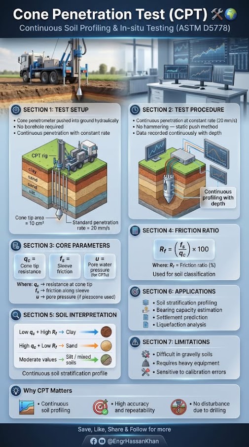
Variables. u2 = pore pressure behind cone tip; an = net area ratio (typically 0.70–0.85, from calibration)
Use. All piezocone (CPTu) soundings; essential in soft clays and silts.
Limitations. Correction negligible in clean sands; critical in soft fine-grained soils. Requires u2 filter position.
Source. Lunne et al. 1997 · In this chapter: 14.15 · Full entry and references
Variables. fs = sleeve friction
Use. All CPT data; basis for SBT classification and most Robertson-family correlations below. Ic < 2.6 ≈ coarse-grained / drained; > 2.6 ≈ fine-grained / undrained.
Limitations. SBT is behaviour type, not grain-size classification. Cemented, aged, or sensitive soils plot misleadingly. Earlier n-exponent forms exist (Robertson & Wride 1998).
Source. Robertson 2009 · In this chapter: 14.6, 14.14, 14.15 · Full entry and references
Variables. Ic from IS-13
Use. Young, uncemented Holocene–Pleistocene soils.
Limitations. Underpredicts Vs in aged or cemented soils. Measure Vs directly for seismic site class.
Source. Robertson 2009 · In this chapter: 14.14 · Full entry and references
Variables. (qc1N)cs = Kc · qc1N; Kc = f(Ic) per Robertson & Wride
Use. Level ground, Mw = 7.5, Ic ≤ 2.6; (qc1N)cs ≥ 160 considered non-liquefiable.
Limitations. For Ic > 2.6, sample and evaluate cyclic softening by lab methods. Thin-layer and transition-zone effects distort qc.
Source. Robertson & Wride 1998; Youd et al. 2001 · In this chapter: 14.6 · Full entry and references
Variables. Ei = intact rock modulus
Use. Based on ~500 in-situ measurements (China, Taiwan).
Limitations. Use simplified form Erm = 100,000 [(1 − D/2)/(1 + e((75+25D−GSI)/11))] MPa only if Ei is unknown.
Source. Hoek & Diederichs 2006 · In this chapter: 14.14 · Full entry and references
Variables. Dn = displacement (cm); ac = critical (yield) acceleration; amax = peak ground acceleration
Use. Rigid-block seismic slope displacement; 2,270 strong-motion records.
Limitations. Rigid-block assumption unsuitable for deep, compliant slides; ±0.510 is one standard deviation in log units. Alternative forms use Arias intensity or magnitude.
Source. Jibson 2007 · In this chapter: 14.0, 14.8, 14.10, 14.15 · Full entry and references
Variables. N = uncorrected SPT blow count (Japanese practice)
Use. All soil types; Japanese database (~1,600 data pairs).
Limitations. Energy basis differs from N60. Standard error is large; use measured Vs (SCPT, MASW, downhole) for site-class or dynamic design.
Source. Imai & Tonouchi 1982 · Full entry and references
Variables. σ'm = mean effective stress; k = 0 (PI=0) to 0.5 (PI ≥ 100)
Use. Uncemented clays and sands; lab resonant-column basis.
Limitations. Underestimates aged/cemented soils; field Vs (Gmax = ρVs2) is preferred.
Source. Hardin 1978 · Full entry and references
Earthquake damage to railroad infrastructure manifests through several mechanisms: embankment slope failures, liquefaction-induced track settlement and lateral spreading, bridge foundation movement, retaining wall failure, and disrupted drainage producing post-event flooding. The consequences range from temporary slow orders to multi-week line closures with significant freight revenue loss.
Railroad seismic design philosophy differs from building or highway design in several important ways:
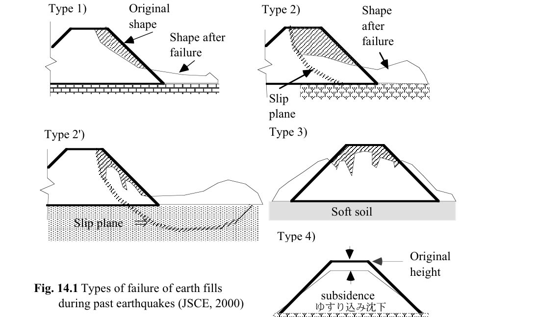
Towhata summarizes the Japan Society of Civil Engineers (JSCE, 2000) classification of residual deformation of road, railway and river-dike fills (Figure 14-S1): Type 1 shallow sliding of the slope surface; Type 2 a slip surface within the fill; Type 2′ a slip surface reaching soft foundation soil; Type 3 slumping (the fill sinks and spreads); and Type 4 densification and subsidence. Faulting directly beneath a fill is a separate case.
Allowable displacement. Because earth structures can be restored far more quickly than steel or concrete, Towhata reports a survey of Japanese infrastructure operators on which observed earthquake displacements they would accept without prior seismic strengthening. Displacements greater than about 6.6 ft were generally not accepted, yet a 33-ft displacement of a railway embankment (Hachinohe) was judged acceptable because it could be restored. Restoration cost did not drive these judgments; effects on the public did. This supports the performance-based tiers in Section 14.1: set the allowable deformation by restoration time and consequence, not a single FS.
Source: Towhata, I. (2008). Geotechnical Earthquake Engineering. Springer
Profillidis frames railway seismic risk in two parts. First, structures, track and subgrade are designed for the regional design acceleration (up to about 10 ft/s² in his text) so that nothing collapses even in the most severe event. In zones of very high seismicity, bridges are fully isolated from their supports with dampers (Figure 14-11). Second, trains are protected during an event by trackside accelerometers that stop traffic above 2.1 ft/s² and reduce speed between 1.3 and 2.1 ft/s² (details in Chapter 4, §4.6).
Figures · click to zoom
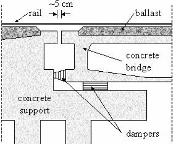
After Profillidis (2014), §9.17, Fig. 9.22. Full reference under Supplemental Sources.
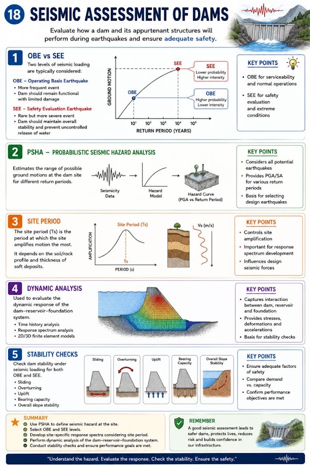
The USGS National Seismic Hazard Model (NSHM) provides the foundation for site-specific hazard characterization. For railroad projects, we access USGS Unified Hazard Tool (https://earthquake.usgs.gov/hazards/interactive/) to extract:
| Railroad Client | FEE (yr) | DE (yr) | MCE (yr) | Primary Standard |
|---|---|---|---|---|
| UPRR | 108 | 475 | 2,475 | UPRR Engineering Instruction Manual — Seismic Design |
| BNSF | 108 | 475 | 2,475 | BNSF Engineering Instructions — Seismic |
| CPKC | 108 | 475 | 2,475 | CPKC Track Standards — Seismic Appendix (legacy CP) |
| Amtrak | 108 | 475 | 2,475 | Amtrak Engineering Standards — Seismic (aligns AASHTO) |
| CN | 108 | 475 | 2,475 | CN Civil Engineering Manual — Seismic Design |
| CSXT | N/A | 475 | 2,475 | CSXT ES — NMSZ Supplement; AASHTO LTS |
| NSR | N/A | 475 | 2,475 | NSR ESM — Bridge Seismic Provisions |
| G&W | N/A | 475 | 2,475 | G&W EB — AREMA Ch. 9 adopted |
| AREMA | N/A | 475 | 2,475 | AREMA MRE Chapter 9 — Earthquake Analysis |
Note: CSXT, NSR, and G&W do not routinely apply the FEE performance level; DE governs new construction.
For structures within 6 miles of a known active fault (e.g., Hayward Fault for UPRR/BNSF Bay Area facilities; Cascadia Subduction Zone for BNSF/UPRR Pacific Northwest mainlines), we supplement PSHA with DSHA: assign maximum magnitude M_max to each fault source, compute median ground motion using attenuation relationships (Campbell-Bozorgnia 2014 NGA-West2 preferred), and compare with PSHA results. The governing hazard level is the greater of the two.
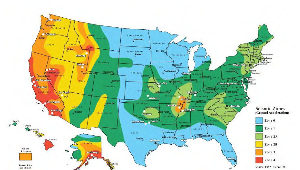
Bridge and wall records from before about 2000 often cite a UBC-style seismic zone (0, 1, 2A, 2B, 3, 4) rather than a PGA. Figure 14-S2 reproduces a commercial version of that map to help interpret those files. Zones were broad bands of approximate ground acceleration and carry no site class, return period or spectral shape, so do not use them for design or screening. Replace them with the USGS NSHM values described above.
Source: Partner Engineering and Science, Inc. Seismic Zone Map of the United States (after the 1997 Uniform Building Code)
Site class is determined from the time-averaged shear wave velocity in the upper 100 ft:
Where:
| Site Class | Description | V_S30 (ft/s) | N̄ (blows/ft) | s̄_u (psf) |
|---|---|---|---|---|
| A | Hard rock | > 5,000 | — | — |
| B | Rock | 2,500–5,000 | — | — |
| BC | Very dense / soft rock | 1,700–2,500 | > 50 | > 5,000 |
| C | Very dense soil / soft rock | 1,200–1,700 | > 50 | > 2,000 |
| CD | Dense soil | 850–1,200 | 30–50 | 1,000–2,000 |
| D | Stiff soil | 530–850 | 15–50 | 1,000–2,000 |
| DE | Soft soil | 365–530 | < 15 | 500–1,000 |
| E | Very soft clay / liquefiable | < 365 | < 15 | < 500 |
| F | Requires site-specific analysis | — | — | — |
Note: ASCE 7-22 uses updated 8-class system (A through F with BC, CD, DE inserted). AASHTO LRFD 9th Ed. retains A–F notation; we reconcile in deliverables.
Reference graphics
Short-period amplification factor (F_a):
Long-period amplification factor (F_v):
Design spectral accelerations:
F_a and F_v are read from ASCE 7-22 Tables 11.4-1 and 11.4-2 as functions of site class and S_S or S_1 at the reference condition. For Site Class E or F, site-specific ground response analysis per ASCE 7-22 Chapter 21 is required. UPRR and BNSF both mandate site-specific response analysis for any Site Class E location along active mainline.
The earthquake-induced cyclic shear stress ratio at depth z (ft) is:
Where:
Stress reduction coefficient r_d (depth z in feet):
The CSR reference condition is M_w = 7.5. For other magnitudes, correct using the Magnitude Scaling Factor (Youd et al. 2001):
| M_w | MSF |
|---|---|
| 5.5 | 2.20 |
| 6.0 | 1.76 |
| 6.5 | 1.44 |
| 7.0 | 1.19 |
| 7.5 | 1.00 |
| 8.0 | 0.84 |
| 8.5 | 0.72 |
The adjusted CSR for comparison with CRR:
For effective stresses exceeding 1 atm (2,117 psf), the cyclic resistance decreases. NCEER recommends:
Where f = 0.7 to 0.8 (conservative practice: use f = 0.7 for coarse sand, 0.8 for fine sand). K_σ ≤ 1.0 and K_σ ≥ 0.5.
For embankment slopes with static shear stress τ_s applied to the failure plane:
Where α = τs / σ'v. For railroad embankments with side slopes 2H:1V to 3H:1V and loose-to-medium dense fill, Kα is read from NCEER (Youd et al. 2001) Figure 10 based on relative density. Kα > 1.0 increases CRR; for loose sands (D_R < 45%) K_α < 1.0 and reduces resistance.
Selig and Waters set out three cyclic failure modes:
Practical consequence. The Seed–Idriss triggering methods in this chapter address earthquake loading. The cyclic softening of a subgrade under traffic is checked differently, using threshold stress and cumulative plastic strain (Chapter 2, §2.4.2). A site can pass one check and fail the other.
After Selig & Waters (1994), ch. 3. Full reference under Supplemental Sources.
Reference graphics
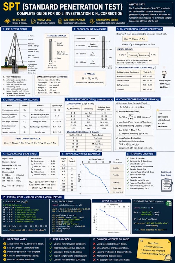
Compute (N₁)₆₀ using the full correction chain established in Chapter 6:
For silty sands (fines content FC > 5%), apply fines correction to obtain the clean-sand equivalent:
Values from these correlations are estimates, not test results. State the equation ID and source when one is used, confirm the soil or rock is within its range, and calibrate against site testing before design.
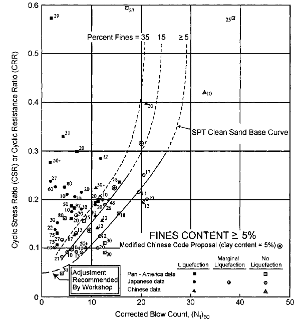
Using the Robertson & Wride (1998) / Youd et al. (2001) relationship for M_w = 7.5:
Valid for (N₁)₆₀,cs < 30. For (N₁)₆₀,cs ≥ 30, the soil is considered non-liquefiable.
Reference graphics · click to zoom
Minimum FS_L acceptance criteria for railroad infrastructure:
| Railroad | FEE Min FS_L | DE Min FS_L | MCE Min FS_L | Governing Standard |
|---|---|---|---|---|
| UPRR | 1.4 | 1.2 | 1.0 | UPRR EIM — Seismic |
| BNSF | 1.4 | 1.2 | 1.0 | BNSF EI — Seismic |
| CPKC | 1.4 | 1.2 | 1.0 | CPKC TS — Seismic Appendix |
| Amtrak | 1.5 | 1.2 | 1.0 | Amtrak ES — Seismic Performance |
| CN | 1.4 | 1.2 | 1.0 | CN ES — Civil Engineering Manual |
| CSXT | N/A | 1.2 | 1.0 | CSXT ES — NMSZ Supplement |
| NSR | N/A | 1.2 | 1.0 | NSR ESM — Bridge Seismic |
| G&W | N/A | 1.2 | 1.0 | AREMA MRE Ch. 9 |
| AREMA baseline | N/A | 1.2 | 1.0 | AREMA MRE Chapter 9 |
Reference graphics
Where n = 0.5 for clean sand; n is refined iteratively using the soil behavior type index I_c (Robertson & Wride 1998):
Start with n = 1.0; compute I_c; update n (n = 0.5 for I_c < 1.64; n = 0.5 + (I_c − 1.64)/3.0 for 1.64 ≤ I_c ≤ 2.60; n = 1.0 for I_c > 2.60); iterate to convergence.
Values from these correlations are estimates, not test results. State the equation ID and source when one is used, confirm the soil or rock is within its range, and calibrate against site testing before design.
For (q_c1N)_cs ≥ 160, the soil is non-liquefiable.
Seed & Harder (1990) correlation with (N₁)₆₀ (SPT-based):
Representative values: (N₁)₆₀ = 5 → s_ur ≈ 100–250 psf; (N₁)₆₀ = 10 → s_ur ≈ 400–900 psf; (N₁)₆₀ = 15 → s_ur ≈ 1,000–2,000 psf. Use lower-bound values for critical structures.
Post-liquefaction slope stability is evaluated with residual strengths substituted for drained strength in Bishop or Janbu analyses (see Chapter 13), checking FS_residual ≥ 1.0 per USACE guidance and ≥ 1.1 per UPRR/BNSF for mainline embankments.
Values from these correlations are estimates, not test results. State the equation ID and source when one is used, confirm the soil or rock is within its range, and calibrate against site testing before design.
Volumetric strain ε_v for saturated sand under cyclic loading is estimated as a function of cyclic shear strain amplitude γ_c and (N₁)₆₀:
Where H_i = thickness of layer i (ft). For a layer with FS_L ≤ 1.0 and (N₁)₆₀ = 10, ε_v is typically 1–3%; for (N₁)₆₀ = 15, ε_v ≈ 0.1–1.0%.
Track geometry acceptance criteria (seismic):
| FRA Track Class | Max Speed (freight) | Allowable Seismic Settlement |
|---|---|---|
| Class 1 | 10 mph | 6.0 in. |
| Class 2 | 25 mph | 4.0 in. |
| Class 3 | 40 mph | 3.0 in. |
| Class 4 | 60 mph | 2.0 in. |
| Class 5 | 80 mph | 1.5 in. |
| Class 6 (Amtrak) | 110 mph | 0.75 in. |
| Class 7 (NEC) | 150 mph | 0.50 in. |
Post-seismic allowable settlement is typically 2× static allowable due to emergency repair expectation.
Reference graphics
The Youd et al. (2002) MLR model estimates horizontal displacement D_H (ft) for free-face and gently sloping ground:
Free-face condition (embankment adjacent to water body):
Gently sloping ground:
Where:
For railroad bridge approaches over rivers and tidal waterways, D_H values exceeding 3 in. typically trigger mitigation requirements for Class 4 and above track.
Fill that has sunk below the water table. The Tokachi River dike in Hokkaido was built in stages over decades on peat (water content about 200%). Much of the fill settled into the peat. Excavation after the 1993 Kushiro-oki earthquake showed that the embankment base had been loosened by that subsidence and lateral spreading and, lying below the water table, was saturated and liquefied. Similar collapses occurred on the Kushiro River dike and the Yodo River dike (1995 Kobe). Railroad embankments built over peat or soft clay and repeatedly raised to restore grade share this geometry. The liquefiable layer may be the old embankment itself, not the natural foundation. Borings through the embankment should log and test the submerged fill “bulb”, not just the native soil beneath it.
Age of the deposit. In Dagupan City (1990 Luzon) and Kobe and Nishinomiya (1995), young hydraulic fill and 20th-century reclamation liquefied while older natural levee deposits and land inside the original shoreline did not. On a rail alignment, historic maps and aerial photos that show where channels, ponds or shorelines were filled are among the cheapest liquefaction screening tools available.
Source: Towhata, I. (2008). Geotechnical Earthquake Engineering. Springer
For seismically induced slope deformation, the Newmark (1965) sliding block method estimates permanent displacement U_d (in.) by integrating the earthquake acceleration record above the critical (yield) acceleration k_y:
Critical (yield) acceleration:
More rigorously, k_y is determined by reducing the pseudo-static coefficient until FS_pseudo = 1.0 in Bishop or Janbu analysis (Chapter 13).
Newmark permanent displacement — Jibson (2007) regression (preferred for engineering practice):
Where U_d is in inches (ln-normal model; reported as median ± 1σ). Alternatively, use Saygili & Rathje (2008) for two-parameter models including PGV.
| U_d (in.) | Performance Interpretation | Action |
|---|---|---|
| < 1.0 | Negligible deformation | No action |
| 1.0–3.0 | Minor; localized cracking expected | Monitor post-event |
| 3.0–6.0 | Moderate; track geometry affected | Remediation or speed restriction |
| > 6.0 | Significant slope movement | Track OOS; remediation required |
| > 12.0 | Slope failure probable | Emergency response; line closure |
Thresholds calibrated to FRA Class 4 track geometry. Amtrak NEC thresholds are 50% of values shown.
Reference graphics
Values from these correlations are estimates, not test results. State the equation ID and source when one is used, confirm the soil or rock is within its range, and calibrate against site testing before design.
| Railroad | Primary Seismic Regions | Liquefaction Screening Trigger | Ground Motion Source | Site-Specific Required? | Notes |
|---|---|---|---|---|---|
| UPRR | Pacific Coast; Wasatch; NMSZ | PGA ≥ 0.10g | USGS NSHM + fault-specific | Yes, Site Class E/F | EIM Seismic Appendix mandatory |
| BNSF | Cascades; Pacific NW; NMSZ | PGA ≥ 0.10g | USGS NSHM | Yes, Site Class E | EI Seismic mandatory; GIS screening tool |
| CPKC | Rocky Mountains; BC Coast | PGA ≥ 0.10g | Geological Survey of Canada | Yes, Site Class E/F | Legacy CP used NBC 2015 |
| Amtrak | NEC (NY–Boston–DC); Pacific NW | PGA ≥ 0.07g | USGS + fault-specific | Yes, all NEC structures | Strictest performance requirements |
| CN | BC Corridor; St. Lawrence | PGA ≥ 0.10g | Geological Survey of Canada | Yes, Site Class E | CN Civil Engineering Manual |
| CSXT | NMSZ; Charleston; Eastern | PGA ≥ 0.15g | USGS NSHM | Yes, new bridges only | NMSZ primary concern |
| NSR | NMSZ fringe; Appalachian | PGA ≥ 0.15g | USGS NSHM | Case-by-case | NSR ESM Bridge Appendix |
| G&W | Regionally variable | PGA ≥ 0.15g | AREMA Ch. 9 / AASHTO | Rarely required | AREMA MRE Chapter 9 adopted |
| AREMA | Varies | PGA ≥ 0.10g | AASHTO site-specific | Ch. 9 guidance | Design basis for Class I adoption |
An automated notification system replaced slow verbal confirmation that once took up to four hours. Events above magnitude 5.0 appear on the rail traffic control terminal with location, size and the required action. Dispatch must acknowledge and print, notify affected movements to stop or run at restricted speed, and await field inspection before restoring normal operations. Criteria differ east and west of 116° longitude because energy carries farther through eastern shield rock.
| Zone | Magnitude | Required action |
|---|---|---|
| East of 116° | 5.0–5.9 | Stop within 50 mi of the epicenter; restricted speed from 50 to 200 mi |
| East of 116° | ≥ 6.0 | Stop within 400 mi |
| West of 116° | 5.0–5.9 | Restricted speed within 50 mi |
| West of 116° | 6.0–6.5 | Stop within 100 mi |
| West of 116° | > 6.5 | Stop within 200 mi |
Restrictions remain until inspections are complete and appropriate speeds are set.
Figures · click to zoom
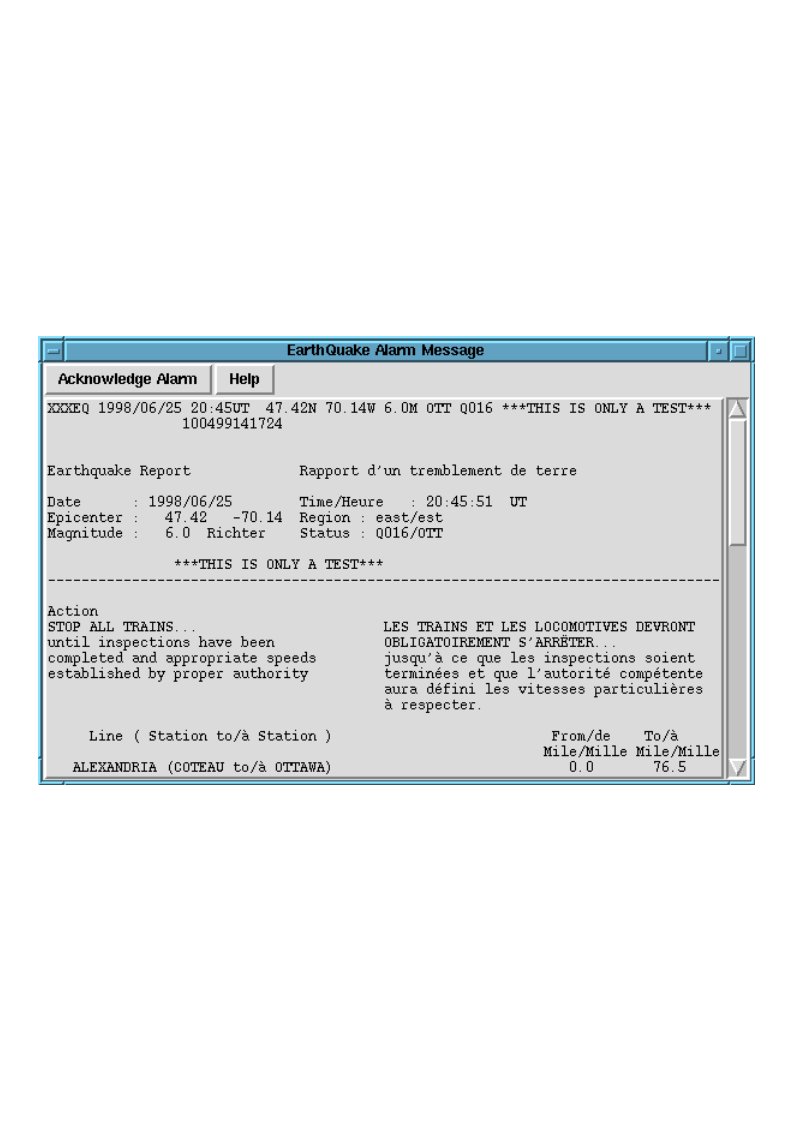
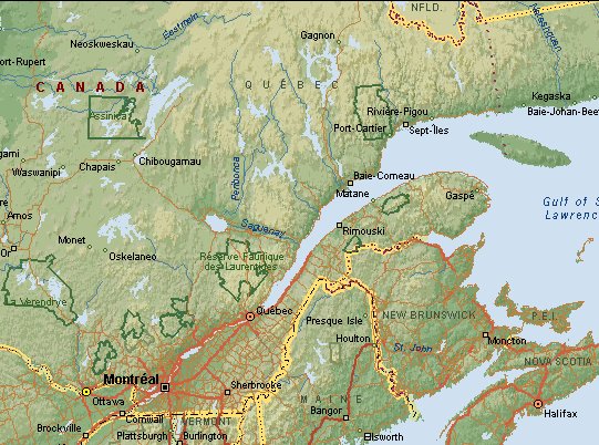
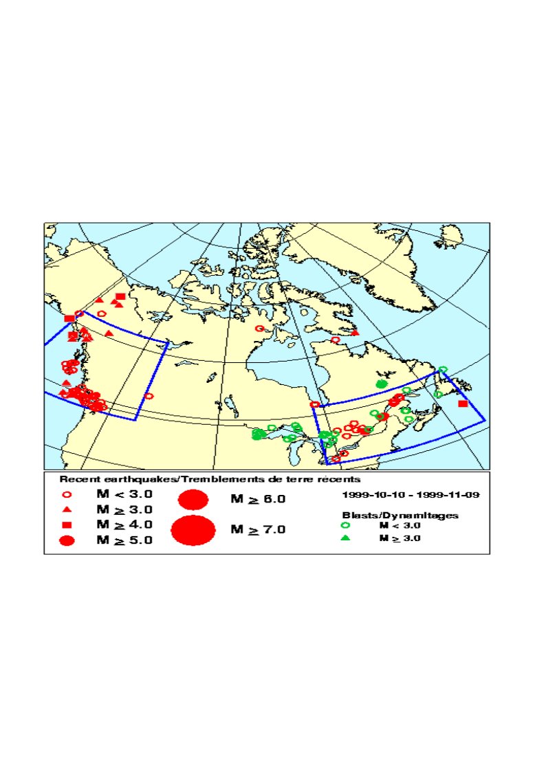
After Geotechnology for Railroaders Program, Module 7.3; §02–04. Full reference under Supplemental Sources.
Worked Example 14-1: Liquefaction Triggering — SPT Method (UPRR Bridge, Cascades)
Project: UPRR bridge replacement over Willamette River tributary, Oregon. M_w = 7.0 design earthquake (Cascadia Subduction Zone). PGA = 0.38g at Site Class B/C (USGS 475-yr return). Site Class D (V_S30 = 660 ft/s).
Soil profile at critical elevation (z = 20 ft):
Step 1 — N₆₀:
Step 2 — C_N and (N₁)₆₀:
Step 3 — Fines correction (FC = 18%):
Step 4 — CRR₇.₅:
Step 5 — CSR:
Site Class D F_a = 1.2 → S_MS = 1.2 × 0.38g = 0.456g → a_max = 0.456g (used for CSR).
Step 6 — MSF (M_w = 7.0):
Step 7 — FS_L:
Interpretation: FS_L = 0.67 < 1.2 (UPRR DE minimum). Liquefaction mitigation required. Estimated seismic settlement (Tokimatsu & Seed): ε_v ≈ 2.5% for (N₁)₆₀ = 17, H = 15 ft → S_seismic ≈ 0.025 × 15 × 12 = 4.5 in., exceeding UPRR Class 4 allowable. Stone column or deep soil mixing remediation recommended.
Worked Example 14-2: Lateral Spreading — CSXT Bridge Approach, NMSZ
Project: CSXT mainline bridge over Obion River, western Tennessee. M_w = 7.7, R = 18 mi from New Madrid Fault. PGA = 0.62g (475-yr USGS). Free-face condition; W = 15% (levee height = 25 ft; distance = 165 ft).
Liquefiable layer characteristics:
Step 1 — Modified source distance:
Step 2 — log D_H (free-face):
log DH = -16.713 + 1.532(7.7) - 1.406 log(34.3) - 0.012(18) + 0.592 log(15) + 0.540 log(22) + 3.413 log(88) - 0.795 log(0.108)
Interpretation: Estimated lateral spreading of 32 ft far exceeds the 3 in. threshold for Class 4 track. This finding is consistent with observed NMSZ lateral spreading up to 50 ft in the 1811–1812 events. CSXT requires deep ground improvement (stone columns or vibro-compaction) to T₁₅ = 0 ft, or alternatively deep pile foundation through liquefiable zone with structural approach slab designed for post-liquefaction differential settlement.
Worked Example 14-3: Newmark Analysis — BNSF Embankment, Pacific Northwest
Project: BNSF embankment slope (H = 28 ft, 2H:1V side slope) at MP 142, Columbia River Gorge. Static FS = 1.65 (Bishop Simplified, drained). PGA = 0.35g (DE, 475-yr). k_y determination required.
Step 1 — Critical acceleration k_y:
Reduce pseudo-static k until FS_pseudo = 1.0:
From Bishop analysis with k_h = 0.0: FS = 1.65. Iterative analysis yields FS_pseudo = 1.0 at k_h = 0.21g → k_y = 0.21g
Step 2 — Newmark displacement (Jibson 2007):
Upper bound (median + 1σ): U_d = 10^{-0.391 + 0.510} = 10^{0.119} = 1.32 in.
Interpretation: Median displacement of 0.41 in. is below BNSF's 1.0 in. threshold (Table 14-5). Upper-bound value of 1.32 in. falls in the "Monitor post-event" range. BNSF accepts this performance level for DE event with post-event inspection protocol activated. No remediation required; embankment is added to BNSF's post-seismic inspection priority list.
Values from these correlations are estimates, not test results. State the equation ID and source when one is used, confirm the soil or rock is within its range, and calibrate against site testing before design.
| Boring | Depth (ft) | N_meas | E_m | N₆₀ | C_N | (N₁)₆₀ | FC (%) | ΔN | (N₁)₆₀cs | CRR₇.₅ | CSR | FS_L | Status |
|---|---|---|---|---|---|---|---|---|---|---|---|---|---|
| B-1 | 10 | 8 | 0.72 | 9.6 | 1.41 | 13.5 | 22 | 5.2 | 18.7 | 0.205 | 0.387 | 0.53 | Liquefiable |
| B-1 | 20 | 14 | 0.72 | 16.8 | 1.20 | 20.2 | 18 | 4.1 | 24.3 | 0.260 | 0.346 | 0.75 | Liquefiable |
| B-1 | 30 | 22 | 0.72 | 26.4 | 1.07 | 28.2 | 8 | 1.8 | 30.0 | NC | 0.316 | NC | Non-liquefiable |
| B-2 | 10 | 6 | 0.72 | 7.2 | 1.41 | 10.2 | 28 | 6.4 | 16.6 | 0.179 | 0.387 | 0.46 | Liquefiable |
| B-2 | 20 | 18 | 0.72 | 21.6 | 1.20 | 25.9 | 12 | 3.2 | 29.1 | 0.310 | 0.346 | 0.90 | Liquefiable |
| B-3 | 10 | 24 | 0.72 | 28.8 | 1.41 | 40.6 | 5 | 0.8 | 41.4 | NC | 0.387 | NC | Non-liquefiable |
| B-3 | 20 | 31 | 0.72 | 37.2 | 1.20 | 44.6 | 3 | 0.4 | 45.0 | NC | 0.346 | NC | Non-liquefiable |
NC = Non-liquefiable ((N₁)₆₀cs ≥ 30). FS_L values < 1.20 flagged for UPRR DE performance requirement.
Values from these correlations are estimates, not test results. State the equation ID and source when one is used, confirm the soil or rock is within its range, and calibrate against site testing before design.
Figure 14-1: USGS Seismic Hazard Map — PGA at 2% PE in 50 yr (2,475-yr return), Western United States, showing UPRR/BNSF/CPKC mainline corridors highlighted.
Figure 14-2: CSR vs. CRR triggering chart (Youd et al. 2001 boundary curve) with plotted liquefaction assessment data from Table 14-7 (liquefiable vs. non-liquefiable points labeled by boring).
Figure 14-3: Stress reduction factor r_d vs. depth (ft) showing three-segment piecewise equation and scatter bounds from Liao & Whitman (1986).
Figure 14-4: Magnitude Scaling Factor (MSF) vs. M_w curve with data points from NCEER Working Group 1996 and Idriss (1999) relationship.
Figure 14-5: SPT-based CRR boundary curve with fines content correction — (N₁)₆₀ vs. CSR₇.₅ showing FC = 0%, 15%, and 35% boundary curves.
Figure 14-6: CPT-based SBT chart (Robertson 1990) with liquefaction susceptibility zones and I_c contours overlaid on representative CPTu sounding from UPRR Cascade corridor.
Figure 14-7: Lateral spreading displacement D_H vs. T₁₅ (Youd et al. 2002 model) for NMSZ M_w = 7.7 scenario — CSXT Tennessee corridor risk map.
Figure 14-8: Newmark displacement vs. k_y/PGA ratio — Jibson (2007) median and ±1σ bounds with BNSF Columbia Gorge embankment case plotted.
Figure 14-9: Typical cross-section showing liquefaction remediation layout — stone column grid pattern with T₁₅ layer identified and design depth annotations.
Figure 14-10: Post-liquefaction failure mechanism schematic for bridge approach embankment — lateral spreading toward channel, settlement trough in track zone, and residual strength failure surface.
Reference graphics



Before instrumental data are available, the Modified Mercalli (MM) intensity describes ground effects that map directly to railroad damage. From the MM descriptions reproduced in Geological Hazards:
| MM | Ground and track effects described |
|---|---|
| VIII | Sand and mud ejected in small amounts; changes in well water |
| IX | Ground cracked conspicuously; underground pipes broken |
| X | Ground badly cracked; rails bent; considerable landslides from river banks and steep slopes; sand and mud shifted |
| XI | Bridges destroyed; broad fissures; earth slumps and land slips in soft ground; rails bent greatly |
Elnashai and Di Sarno list rail bending or rupture and derailment among the typical earthquake damage to highway and railway lifelines, along with pier failure, unseating at bearings and pavement cracking and settlement. They also note that lurch cracking of soft saturated ground and movement toward steep slopes and cliffs damage transportation corridors even away from the fault. Intensity scales differ internationally (Figure 1.13 in Elnashai compares MM, MCS, MSK, EMS and the 7-level JMA scale), so convert when using foreign reconnaissance reports.
Numerical models of two integral-abutment bridges (13 variants each, with dense to loose sand and stiff to soft clay around the piles) found that replacing compacted backfill with EPS geofoam reduced seismic moment and shear in the integral abutments in every case. The cost was slightly larger abutment and pier displacement and somewhat higher pier forces, which the author judged designable. For railroad structures in moderate seismic zones, the same approach can reduce abutment demand. Check the added displacement against track tolerances, and see Chapter 12 for geofoam properties and buoyancy.
Source: Elnashai, A. S. and Di Sarno, L. (2008). Fundamentals of Earthquake Engineering. Wiley · Bolt, B. A., Horn, W. L., Macdonald, G. A. and Scott, R. F. (1977). Geological Hazards: Earthquakes, Tsunamis, Volcanoes, Avalanches, Landslides, Floods, 2nd ed. Springer-Verlag
Values from these correlations are estimates, not test results. State the equation ID and source when one is used, confirm the soil or rock is within its range, and calibrate against site testing before design.
Checklist · Part VI · Geotechnical Analysis
Pre-Field / Desktop Phase
Field Investigation Phase
Analysis Phase
Deliverable Phase
Values from these correlations are estimates, not test results. State the equation ID and source when one is used, confirm the soil or rock is within its range, and calibrate against site testing before design.
Question 9-1: A SPT boring in southern Illinois (NMSZ zone, M_w = 7.7, PGA = 0.50g at rock, Site Class D, F_a = 1.2) shows N_meas = 10 blows/ft at z = 15 ft. Total unit weight γ = 118 pcf; WT at z = 4 ft. Hammer energy E_m = 0.72; C_B = 1.0; C_R = 0.85; C_S = 1.0. FC = 20%. Compute FS_L.
Answer 9-1:
Question 9-2: A BNSF site in central Washington has V_S30 = 780 ft/s. What is the ASCE 7-22 site class? If S_S = 1.25g and F_a = 1.0 (Site Class D), what is S_DS?
Answer 9-2:
Question 9-3: A Amtrak NEC embankment (Class 7 track) overlies 8 ft of loose sand (FS_L = 0.72, (N₁)₆₀ = 9) at z = 10–18 ft. Estimate seismic settlement using Tokimatsu & Seed (1987). Is this acceptable for Amtrak service?
Answer 9-3:
Question 9-4: A slope at a CPKC Rockies location has k_y = 0.15g and PGA = 0.30g at the DE level. Using Jibson (2007), compute the median Newmark displacement and assess acceptability.
Answer 9-4:
Question 9-5: A CPTu sounding at a CSXT Mississippi Delta site shows q_c = 25 tsf (526,000 psf), f_s = 0.30 tsf (6,300 psf), u₂ = 0.04 tsf (840 psf), at z = 12 ft with σ_v = 1,380 psf, σ'_v = 840 psf. Compute I_c (initial iteration, n = 1.0) and assess soil behavior type.
Answer 9-5:
Values from these correlations are estimates, not test results. State the equation ID and source when one is used, confirm the soil or rock is within its range, and calibrate against site testing before design.
| Topic | Refer To |
|---|---|
| SPT N₆₀ and (N₁)₆₀ calculation procedure | Chapter 6, Section 6.3 |
| CPTu q_t correction and SBT classification | Chapter 7, Section 7.2 |
| MASW for V_S30 determination | Chapter 7, Section 7.6 |
| Groundwater measurement and seasonal monitoring | Chapter 9, Sections 9.2–9.3 |
| Slope stability — pseudo-static and residual strength | Chapter 13, Sections 13.4 and 13.9 |
| Embankment settlement under surcharge | Chapter 12, Section 12.4 |
| Ground improvement for liquefiable zones | Chapter 17 |
| Construction monitoring for ground improvement | Chapter 15, Section 15.5 |
| GDR documentation of seismic findings | Appendix E, Section E.4 |
| Laboratory grain size and fines content | Chapter 10, Sections 10.2–10.3 |
End of Chapter 14 — Seismic Hazard and Liquefaction
Authors: Daniel P. Colwell and Mario Ruel. This chapter was written and compiled by Daniel P. Colwell and Mario Ruel for Railway Ground Hazard Risk Management.
Technical content is drawn from the published sources below, and credit for that material belongs to their authors and publishers. Tables, equations and figures taken from a specific source are also cited where they appear.
File locations for these documents are listed under Supplemental Sources — LEVI Library.
Material in the green “Supplemental reference” boxes throughout this chapter was added from the following documents in the LEVI geotechnical library. Text is summarized or paraphrased; tables are reproduced with their original source noted; figures are reproduced from the cited document for internal reference use. Consult the original document before relying on a value for design. Blocks marked “After Selig & Waters (1994)” summarize item S8 for railroad clients; tables are condensed from the book and its figures are not reproduced.