
Geotechnical engineering libraryContact
 benesch
Primary Reference: USACE EM 1110-1-1804, Geotechnical Investigations (2001), Sections 5-1 through 5-8; USACE EM 1110-2-1901, Seepage Analysis and Control for Dams (1993); ASTM D1586, D4750, D4044, D2434, D5084, D5856; AREMA MRE Chapter 1, Sections 1.3–1.4; FHWA HEC-18 (Scour at Bridges).
Railroad Standards: CSXT Engineering Standards — Drainage and Earthwork; NSR Engineering Standards Manual §4.1 (Drainage); G&W Engineering Bulletins — Drainage and Culverts; UPRR Engineering Instruction Manual §DR-100; BNSF Engineering Instructions — Drainage; CPKC Track Standards — Drainage; Amtrak Engineering Standards — Drainage and Seepage; CN Engineering Standards — Drainage and Hydrology.
Apps on dirtbert.com that support this chapter. Each one runs in a web browser on a desktop or a phone, with nothing to install. How to use the apps (I.3). Tools marked TOOLS open in the Geotechnical Analysis Suite (Benesch sign-in); the orange card below lists each one by section.
NANCY pages ask you to accept the Use and Disclaimers once in each browser. MINA is a monitoring aid and is not for operational dispatch decisions.
Calculators and workbook tools from the Benesch Geotechnical Analysis Suite that support this chapter: 1 interactive calculator and 6 workbook guides. Each one is also placed inside the section it supports, in an orange tools strip.
| GW | Infiltration Calculations & ProcedureUsed in 9.4 Field Permeability Testing | Calculator ▸ | Guide |
| GW | Slug Test — Bouwer–RiceUsed in 9.4 Field Permeability Testing | guide only | Guide |
| GW | Slug Test — HvorslevUsed in 9.4 Field Permeability Testing | guide only | Guide |
| GW | Seepage Through Dam (Kozeny)Used in 9.5 Seepage Analysis | guide only | Guide |
| GW | UnderseepageApplies to the chapter as a whole | guide only | Guide |
| GW | Falling Head Tube CalibrationsUsed in 9.4 Field Permeability Testing | guide only | Guide |
| GW | Well Construction Summary (BRLF)Used in 9.3 Piezometers — Types, Installation, and Monitoring | guide only | Guide |
Tools open on dirtbert.com and need the Benesch sign-in. Drafts pending Benesch final review, not for use in design.
General topic illustrations from Benesch's shared geotechnical graphics library, related to this chapter's subject matter — not the numbered figures called out in the text above. Click any image to view it full size.
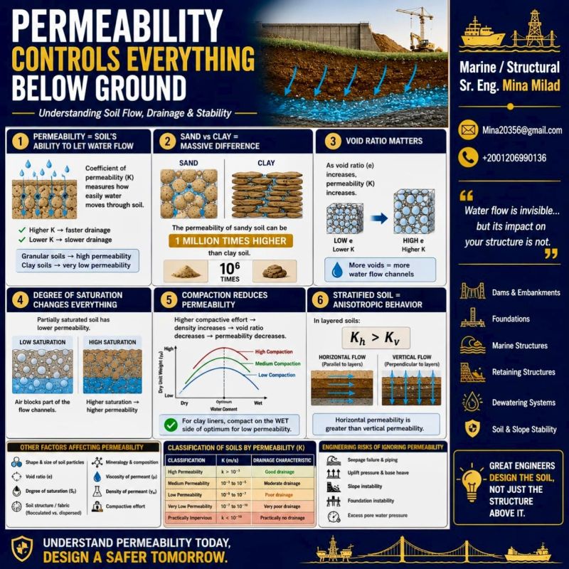
Groundwater is the single most consequential subsurface variable in railroad geotechnical engineering. It controls effective stress — and therefore bearing capacity and slope stability — in every analysis we perform for CSXT, NSR, UPRR, BNSF, CPKC, Amtrak, CN, and G&W clients. It governs embankment drainage design, subgrade softening potential, frost action severity, scour vulnerability at bridges, and dewatering requirements during construction. Despite its importance, groundwater is the most commonly undercharacterized parameter in railroad geotechnical investigations: single-point water level readings taken during drilling, without stabilization time or seasonal monitoring, have caused more railroad geotechnical design failures than any other data deficiency we encounter in practice.
This chapter establishes how we characterize groundwater for railroad clients — from initial observations during drilling through seasonal piezometer monitoring programs, field permeability testing, seepage analysis, and dewatering design. All equations, examples, and tables use English units (psf, pcf, ft/day, ft/s, ft). Cross-references to Chapters 11 (bearing capacity), 7 (settlement), 8 (slope stability), and 9 (seismic/liquefaction) highlight where groundwater inputs from this chapter directly drive design outcomes.
The correlations below are used or referenced in this chapter. Each is a statistical fit to a particular data set, so a value from one is an estimate: it applies only within the materials and ranges stated, carries the scatter of the original data, and must be confirmed by site-specific testing or calibration before it is relied on for design.
When an equation is used, note it with the result: give the equation ID and source, state that the soil or rock is within its range of applicability, mark the value as correlated (not tested), and record the limitation that governs. The Empirical Equations & Correlations reference has every entry with its full references.
Variables. D10 = effective grain size
Use. Loose, clean, uniform sands (Cu < ~5); D10 ≈ 0.1–3 mm.
Limitations. Ignores density and fabric. Errors of an order of magnitude are common in silty or well-graded soils.
Source. Hazen 1911 · Full entry and references
Variables. e = void ratio
Use. Natural, non-plastic sands and gravels; developed for roughly 0.003 < D10 < 3 mm and 0.3 < e < 1.0.
Limitations. Typical accuracy within a factor of about 2–3 in clean soils. Not for plastic fines or cohesive soils.
Source. Chapuis 2004 · Full entry and references
Variables. Ic from IS-13
Use. Naturally deposited soils; first-order profiling of k with depth.
Limitations. Order-of-magnitude only (±1 log cycle). Not for man-made fills; prefer CPTu dissipation t50 or field pumping tests for design.
Source. Robertson 2010 · Full entry and references
Reference graphics · click to zoom
The fundamental relationship between groundwater and geotechnical performance is governed by effective stress (Terzaghi 1936):
Reference graphics
Water reaches the track substructure from three sources:
Subballast and subgrade perform best somewhere between dry and saturated.
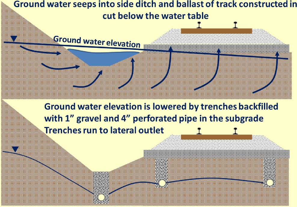
Groundwater is mainly a problem in cuts, where the water table stood above the excavation level before the cut was made. There it causes seepage, erosion and instability in the slopes, and upward seepage into the track. Embankments and level ground with the water table below the surface are not affected by seepage unless there is artesian pressure. Capillary water can still weaken a fine-grained subgrade and feed ice lenses.
Time and drainage. Partial drainage and the rest periods between trains slow the build-up of pore pressure under traffic. Fine-grained subgrade that starts nearly saturated, with limited drainage, approaches full saturation and responds undrained. Expect seasonal changes in response as saturation varies.
After Selig & Waters (1994), chs. 3 and 13. Full reference under Supplemental Sources.
σ'_v = σ_v − u
Where:
When the water table rises — seasonally, due to heavy rainfall, or due to a blocked drainage culvert — pore pressure increases, effective stress decreases, and the shear strength and stiffness of the soil decrease. For a railroad embankment, this directly translates to:
Each of our nine railroad clients has a distinct groundwater risk profile shaped by geography, geology, and operational history:
CSXT — Atlantic Coastal Plain corridors (Virginia, North Carolina, South Carolina, Georgia, Florida): shallow water tables typically 2–6 ft below grade; seasonal fluctuations of 3–8 ft; tidal influence near coastal crossings; artesian pressures in Cretaceous confined aquifers beneath Piedmont corridors. CSXT Engineering Standards require seasonal high water table to be used as the design groundwater level for all embankment and subgrade analyses.
NSR — Appalachian Mountain routes (Virginia, West Virginia, Kentucky, Tennessee): fractured rock aquifers; perched water tables on ridge slopes; springs and seeps at bedrock outcrop locations; slope instability risk driven by elevated phreatic levels in residual soils. NSR's Engineering Standards Manual §4.1 requires piezometer installation at every cut slope investigation that will be used in a slope stability analysis.
UPRR — Great Plains and Intermountain West: deep water tables (20–100 ft) in semi-arid regions; confined artesian aquifers under alluvial valley fills in the western United States; expansive clay subgrades subject to shrink-swell rather than saturation-driven failure; loess collapsibility triggered by wetting. UPRR Engineering Instruction Manual §DR-100 requires groundwater depth to be confirmed by a 24-hour stabilized reading, not just drilling observation.
BNSF — Pacific Northwest and Northern Plains: seasonal flooding risk along river corridors; elevated water tables in Pacific Northwest rain shadow regions; artesian conditions in glacial lake sediment sequences across Montana and the Dakotas; scour-critical bridge sites throughout the Missouri and Columbia River drainages. BNSF Engineering Instructions require annual scour monitoring reports for designated scour-critical bridges.
CPKC — Canadian Prairie: shallow water tables in glaciolacustrine clay deposits; spring snowmelt saturation cycles that reduce subgrade strength to critical levels annually; permafrost-adjacent conditions north of approximately 54°N in Alberta and Saskatchewan. CPKC Track Standards require spring thaw load restrictions to be coordinated with seasonal groundwater monitoring data.
Amtrak — Northeast Corridor: tidal and estuarine groundwater in New Jersey and Maryland coastal segments; high water tables in Baltimore and Philadelphia fill areas; historic railroad fill containing coal ash, cinders, and debris that alters drainage; artesian pressures in confined sand lenses beneath Potomac clay deposits along the Washington DC segment. Amtrak Engineering Standards require long-term (minimum 1 year) seasonal monitoring on any NEC project where groundwater is within 8 ft of the top of subgrade.
CN — Great Lakes and Laurentian Shield: perched water in glacial till; lacustrine clay deposits with elevated pore pressures from recent unloading (post-glacial rebound); muskeg peat deposits with high water retention; permafrost-adjacent conditions across northern Ontario and Quebec. CN Engineering Standards require that groundwater characterization distinguish between perched, unconfined, and confined aquifer conditions in glaciated terrain.
G&W — Mississippi Delta and Gulf Coast: near-surface water tables within 1–3 ft of grade; artesian pressures in Miocene confined aquifers beneath thick clay sequences; tidal influence in Louisiana and Mississippi bayou crossings; rapid seasonal fluctuation in response to heavy rainfall events. G&W Engineering Bulletins require that groundwater levels be confirmed by monitoring during both dry-season (summer) and wet-season (late winter / spring) field programs.
In the UIC subgrade classification, hydrogeological conditions are the second fundamental parameter after soil type: the same soil moves down a class when they are “bad” (Chapter 2, §2.4). The UIC guidance is that groundwater should stay at least 2.6 ft below the top of subgrade, lowered by ditches or deep drains where necessary. Railways set their own minimum depths below rail or formation level (Figure 9-9). Conditions are still not rated good without drainage devices and a 3–5% crossfall on the subballast. Areas with large groundwater fluctuation need a separate study, and a sand filter or geotextile may be justified.
This makes the seasonal high groundwater level, not the level on the day of drilling, the value that governs subgrade classification. Plan piezometer readings to capture it.
Figures · click to zoom
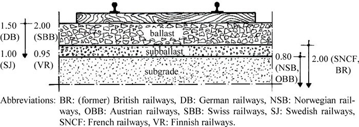
After Profillidis (2014), §9.4, §9.14.1, Fig. 9.3. Full reference under Supplemental Sources.
Two water level observations are recorded in every boring:
Reference graphics
h = z_m + y_w
Where:
Artesian pressure occurs when the piezometric head at a confined aquifer exceeds the ground surface elevation. Artesian conditions are common beneath the Cretaceous and Paleogene clay confining layers that underlie CSXT and NSR coastal plain corridors, beneath glacial lake clay sequences in CN's Great Lakes Division, and beneath valley fill alluvium in BNSF's mountain subdivision river crossings.
Recognition during drilling: When drilling into a confined aquifer, water rises rapidly in the borehole and may overflow the top of casing. The drill crew must be instructed to record the overflow rate and borehole water level carefully. An overflowing borehole indicates artesian head = ground surface elevation + any additional head above the casing top.
u_artesian = γ_w × (h_piezometric − z_ground surface) = 62.4 × Δh
Where Δh = height of artesian water above ground surface (ft). Artesian conditions reduce effective stress to zero at the confining layer base, eliminating bearing capacity in the overlying material — a critical finding that must be flagged immediately to the railroad project manager.
The open standpipe piezometer is the simplest and most robust device for long-term water level monitoring in railroad geotechnical programs. A perforated PVC screen is installed at the desired monitoring depth; solid PVC casing extends to the surface; sand filter pack surrounds the screen; bentonite seal prevents vertical communication between aquifer zones.
Installation procedure:
Measurement: Electronic water-level indicator (e-tape) or steel tape weighted with chalk. Read to nearest 0.01 ft. Record measurement point elevation (top of casing or top of protective cap) surveyed to NAVD 88.
Response time: Hours to days in sands and gravels; days to weeks in silts; weeks to months in clays. Open standpipes are generally NOT suitable for real-time monitoring in clay — use pneumatic or vibrating wire transducers instead.
Vibrating wire (VW) transducers provide real-time pore pressure monitoring via a continuously tensioned wire whose resonant frequency changes with applied pressure. Data is transmitted via cable or wireless logger. Applications:
u (psf) = [G × (f_r² − f_0²) + C_T × ΔT] × 144
Where:
Pneumatic transducers use compressed gas to measure pore pressure via a pneumatic circuit. They are simpler and less expensive than VW instruments but do not provide real-time data logging. Used on NSR and G&W projects where periodic manual readings are acceptable and budget constraints limit the use of automated instrumentation.
| Client | Minimum Monitoring Duration | Reading Frequency | Trigger for Extended Monitoring |
|---|---|---|---|
| CSXT | 3 months (dry) + 3 months (wet) | Weekly | Any reading > 3 ft rise between sessions |
| NSR | 1 full calendar year for slopes | Monthly (minimum) | Seasonal fluctuation > 5 ft |
| UPRR | 24-hr stabilized minimum; 6 months if seasonal data needed | Weekly during monitoring | Water table < 6 ft below subgrade |
| BNSF | 6 months including spring snowmelt period | Bi-weekly | Spring rise > 4 ft |
| CPKC | 1 full year in Canadian prairie | Monthly; bi-weekly during spring thaw | Frost thaw saturation events |
| Amtrak | 1 year minimum on NEC soft-ground projects | Weekly; daily during major rain events | B_q > 0.4 in CPTu data |
| CN | 1 year on projects with soft clay or muskeg | Monthly; bi-weekly during spring thaw | Leda clay or quick clay identified |
| G&W | 2 seasons (dry + wet) minimum | Bi-weekly | GWT within 3 ft of subgrade |
Reference graphics
Slug tests estimate the hydraulic conductivity (k) of the soil or rock at the piezometer screen interval by measuring the rate of water level recovery after a sudden injection or withdrawal of a known volume.
k = [r_c² × ln(R_e / r_w)] / [2 × L_e × t] × ln(y_0 / y_t)
Where:
Plot ln(y_t/y_0) vs. t; slope = −k × 2L_e / [r_c² × ln(R_e/r_w)].
For granular soils in the laboratory:
k = Q × L / (A × Δh × t)
Where:
No additional content.
k = (a × L / A × t) × ln(h₁ / h₂)
Where:
For aquifer characterization on major railroad projects requiring dewatering design:
T = 2.303 × Q / (4π × Δs)
Where:
k = T / b
Where b = saturated aquifer thickness (ft).
S = 2.25 × T × t₀ / r²
Where t₀ = time intercept where the Cooper-Jacob straight line intersects s = 0 on the time axis (days), and r = distance to observation well (ft).
| USCS Symbol | Soil Type | k (ft/day) | k (ft/s) |
|---|---|---|---|
| GW, GP | Clean gravel | 100 – 3,000 | 1.2×10⁻³ – 3.5×10⁻² |
| SW, SP | Clean sand | 10 – 300 | 1.2×10⁻⁴ – 3.5×10⁻³ |
| SM | Silty sand | 0.3 – 10 | 3.5×10⁻⁶ – 1.2×10⁻⁴ |
| ML | Silt | 0.003 – 0.3 | 3.5×10⁻⁸ – 3.5×10⁻⁶ |
| CL | Lean clay | 0.0003 – 0.01 | 3.5×10⁻⁹ – 1.2×10⁻⁷ |
| CH | Fat clay | < 0.0001 | < 1.2×10⁻⁹ |
| Fractured rock | Variable | 0.03 – 300 | 3.5×10⁻⁷ – 3.5×10⁻³ |
GEC 5 recommends estimating k from soil type and grain size before reducing test data, then treating any discrepancy of more than about two orders of magnitude as a sign of test error or unusual soil. Hazen’s equation, k (cm/s) = C·d102 with C = 0.4–1.2 and d10 in mm, applies only to clean sands (< 5% passing No. 200, d10 = 0.0039–0.12 in.). Against slug tests in an alluvial sand aquifer, its error ranged from slight to more than one order of magnitude.
Robertson and Cabal (2010) relate k to the soil behavior type index: k = 10(0.952 − 3.04 Ic) m/s for 1.0 < Ic ≤ 3.27, and k = 10(−4.52 − 1.37 Ic) m/s for 3.27 < Ic < 4.0. The relationship is approximate, but a CPTu profile shows thin pervious seams between piezometer screens that point tests miss. For soft clays (after Jamiolkowski et al., 1985) kh/kv is about 1–1.5 for homogeneous deposits, 2–4 for sedimentary clays with discontinuous pervious lenses, and 3–15 for varved clays with continuous pervious layers — the ratio needed for the transformed flow-net section above.
Source: Sabatini, P. J. et al. (2002). Evaluation of Soil and Rock Properties. Geotechnical Engineering Circular No. 5, FHWA-IF-02-034 · Robertson, P. K. and Cabal, K. L. (2010). Guide to Cone Penetration Testing for Geotechnical Engineering, 4th ed. Gregg Drilling & Testing
No additional content.
i = Δh / L
Where Δh = head loss (ft) and L = seepage path length (ft).
v = k × i
v_a = k × i / n
Where n = porosity (dimensionless); typical values: gravels 0.25–0.40; sands 0.30–0.45; silts 0.35–0.50; clays 0.40–0.70.
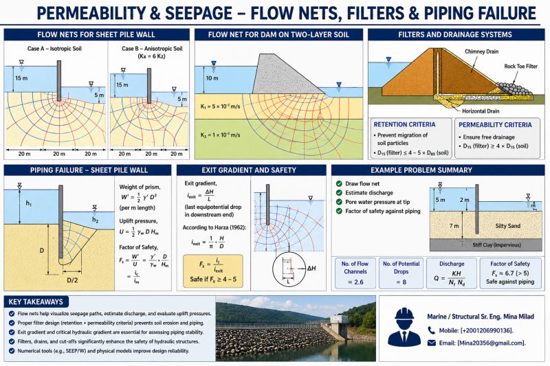
For embankment seepage with a defined flow net (N_f flow channels, N_d equipotential drops):
Reference graphics
q = k × H × (N_f / N_d)
Where H = total head loss (ft); q = seepage flow per unit width of embankment (ft²/day).
AREMA MRE Chapter 1 §1.4 requires that embankments over 15 ft high adjacent to waterways be evaluated for seepage using a flow net or numerical analysis when site-specific soil permeabilities are available. BNSF Engineering Instructions require seepage analysis for all embankments within 200 ft of a waterway designated as a scour-critical bridge approach.
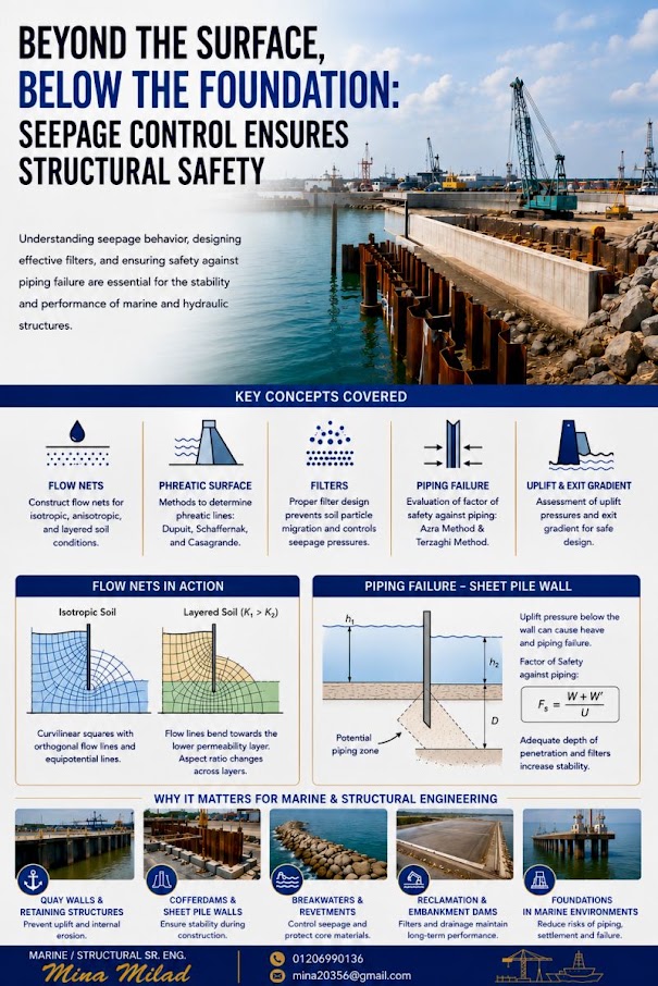
Upward seepage beneath a railroad embankment or at the toe of a flood-side levee can cause piping or heave when the upward seepage force exceeds the submerged weight of soil:
i_cr = (G_s − 1) / (1 + e) = γ' / γ_w
Where:
For a typical medium sand (G_s = 2.65, e = 0.65):
i_cr = (2.65 − 1) / (1 + 0.65) = 1.65 / 1.65 = 1.00
FS_piping = i_cr / i_exit
USACE EM 1110-2-1901 requires FS_piping ≥ 4.0 for permanent railroad embankments adjacent to waterways. BNSF Engineering Instructions reference this criterion for all bridge approach embankment designs on scour-critical corridors.
AREMA MRE Chapter 8 requires scour analysis at all waterway crossings per FHWA HEC-18. Total scour depth:
Reference graphics
Reference graphics · click to zoom
y_total = y_long + y_contr + y_local
Where:
y_s / y_1 = 2.0 × K₁ × K₂ × K₃ × K₄ × (a/y_1)^0.65 × Fr₁^0.43
Where:
Scour analysis results are submitted to BNSF, UPRR, NSR, CN, and CPKC bridge engineering departments as part of the scour evaluation report required annually for scour-critical bridges per FHWA Bridge Inspector's Reference Manual.
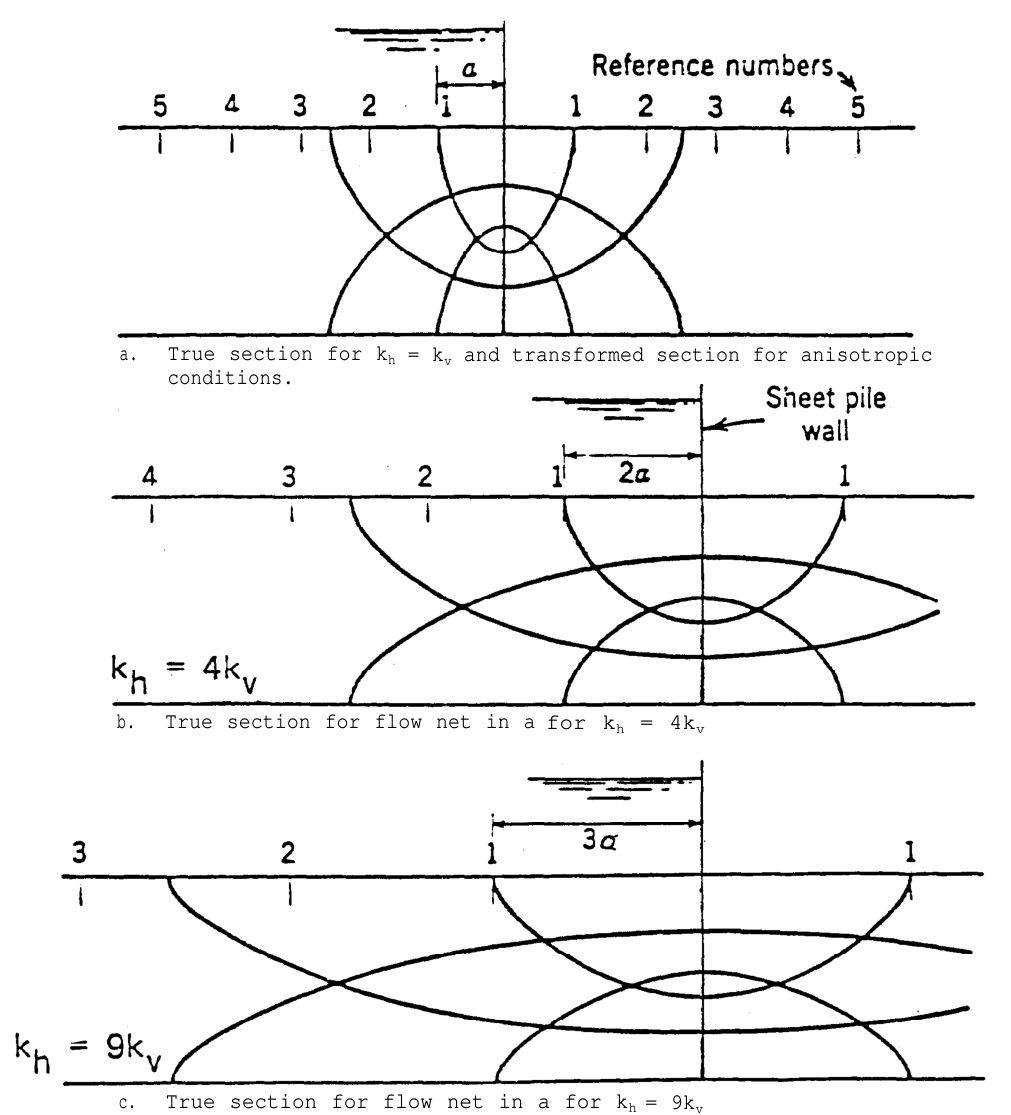
Water-laid soils are usually more permeable horizontally than vertically (wind-blown silts can be the reverse because of root holes). A flow net is only valid for isotropic conditions, so USACE draws it on a transformed section: multiply every horizontal dimension by √(kv/kh), draw a square flow net, then map it back to the true section. Seepage quantity uses the equivalent permeability k′ = √(khkv). Pore pressures and uplift can be read from either section, but gradients and seepage forces must be taken from the true section — the exit gradient in Eq. 9-16 is understated if it is scaled from the transformed net. Figure 9-S1 shows the same net for kh = kv, 4kv and 9kv.
At boundaries between soils of different permeability, flow channels narrow and equipotential spacing widens as water passes into the more permeable layer — head is lost mainly in the tighter soil.
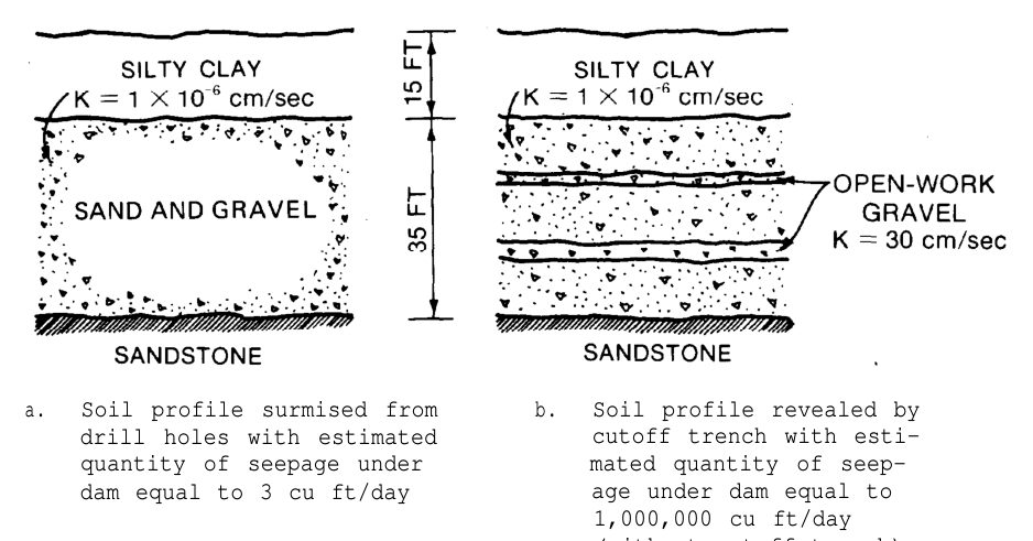
USACE cites Cedergren’s case of a dam foundation logged from borings as uniform sandy gravel: lab tests on disturbed samples gave k ≈ 3 × 10⁻³ ft/day and a predicted underseepage of 3 ft3/day. The cutoff trench exposed streaks of openwork gravel (k ≈ 85,000 ft/day); without the cutoff, seepage would have been about 1,000,000 ft3/day. Grain-size sampling in drill holes washes out the very feature that controls flow. For railroad embankments beside rivers and at bridge approaches in alluvial gravel, rely on pumping tests and groundwater response to river stage, not lab permeability of disturbed samples. The reverse is also true: a thin continuous clay seam can control vertical flow through an otherwise pervious site.
Source: U.S. Army Corps of Engineers (1986, Change 1 1993). Seepage Analysis and Control for Dams. EM 1110-2-1901
A drain at the toe of an embankment, behind a wall, or around an edge-drain pipe must keep the protected soil in place while passing water. USACE EM 1110-2-1901 (App. D, adopted from the NRCS 1986 filter guide) sizes the filter from the protected (“base”) soil:
Table 9-S1. USACE filter criteria (d = base soil, D = filter)
| Base soil category | % finer than No. 200* | Retention criterion |
|---|---|---|
| 1 – fine silts and clays | > 85 | D15 ≤ 9 × d85 |
| 2 – sands, silts, clays, silty/clayey sands | 40–85 | D15 ≤ 0.028 in. |
| 3 – silty and clayey sands and gravels | 15–39 | D15 ≤ [(40 − A)/(40 − 15)] × [(4 × d85) − 0.028 in.] + 0.028 in. (A = % passing No. 200) |
| 4 – sands and gravels | < 15 | D15 ≤ 4 to 5 × d85 |
* After regrading the base soil on the minus No. 4 fraction when it contains gravel.
These criteria are more specific than the Terzaghi ratios used for subballast in Chapter 2 and are the ones to cite for edge drains, wall drains and toe filters in railroad embankments.
Source: U.S. Army Corps of Engineers (1986, Change 1 1993). Seepage Analysis and Control for Dams. EM 1110-2-1901
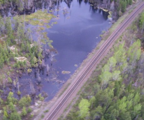
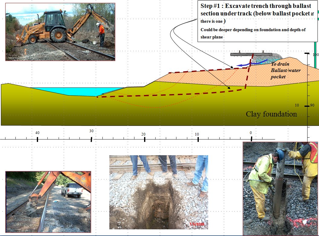
A head difference of more than about 6 ft across an embankment forces flow beneath the track. Seepage zones appear at the downhill toe within days, depending on fill permeability. Thin, permeable granular layers hidden in a fill can carry water deep into it unseen; an April 2013 slope failure followed exactly that path from a wet uphill ditch. Dirty or milky water and sand fans mean piping is underway. When seepage appears, do not plug it with clay. Let it out through ballast, geotextile and gravel so pressure cannot build.
Figures · click to zoom
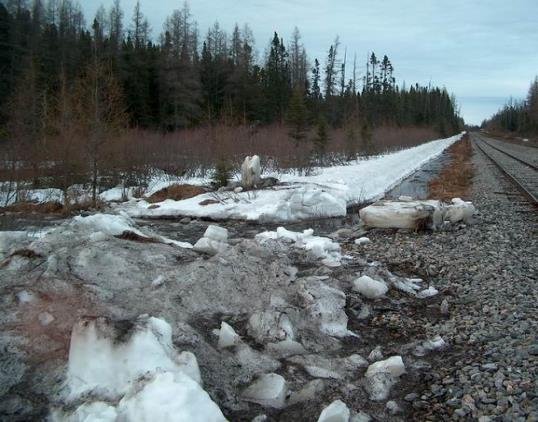
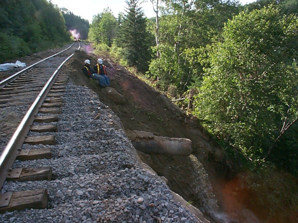
After Geotechnology for Railroaders Program, Module 7.1, Module 4, Module 2; Module 7.1 §04–05; Module 4 §08; Module 2 §06. Full reference under Supplemental Sources.
When railroad construction requires excavation below the water table — for bridge footing construction, retaining wall foundation placement, or culvert installation — dewatering is required. Our geotechnical investigation provides the hydraulic conductivity and aquifer geometry data that the dewatering contractor uses to design the system.
| Method | Best For | k Range (ft/day) | Max Drawdown |
|---|---|---|---|
| Sump pumping | Gravels, cobbles | > 1,000 | Unlimited if pump capacity adequate |
| Wellpoints | Sands, silty sands | 1 – 100 | 15–18 ft per stage |
| Deep wells | Confined aquifers, deep drawdowns | 0.1 – 1,000 | Unlimited |
| Eductor wells | Silts, fine sands | 0.001 – 1.0 | 50–100 ft |
| Horizontal drains | Slope drainage, moderate k | 0.01 – 10 | N/A |
| Electro-osmosis | Clays | < 0.001 | Limited |
CSXT Engineering Standards require dewatering plans to be submitted to CSXT's Environmental group when construction is within 100 ft of a waterway or wetland. UPRR EIM §DR-100 requires a dewatering permit application and groundwater monitoring plan before construction dewatering begins within UPRR right-of-way.
Reference graphics
For a wellpoint system, the required spacing is estimated from:
Q_w = π × k × H_w² / (2 × ln(R_e / r_w))
Where:
R_e = 3,280 × H_w × √k
Where H_w in ft and k in ft/s. Result in ft.
Figures · click to zoom
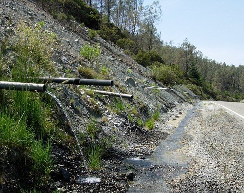
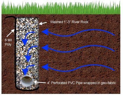
After Geotechnology for Railroaders Program, Module 6.1, Module 6.2, Module 4; Module 6.1 §02; Module 6.2 §02; Module 4 §05. Full reference under Supplemental Sources.
Smith and Hinze write from the general contractor’s side, cataloguing scope items that tend to fall between subcontracts. They note that sizing wells to the water table handles most of the inflow, but the remainder often comes from conditions the borings missed, such as a perched sand layer over clay or rock feeding water through the lagging. They also note that dewatering cost is rarely obvious from the drawings, so a contingency for spot dewatering is prudent. Their checklist includes:
For railroad work: Culvert replacements, bridge foundation work and cut-and-cover crossings under or beside live track add a consequence the building-site checklist does not: loss of dewatering can soften the embankment or subgrade carrying traffic, not just the excavation bottom. In the dewatering GSP and the monitoring plan:
Coordinate discharge routing with the railroad’s drainage and environmental staff, since ditches along the right-of-way often discharge to regulated waters.
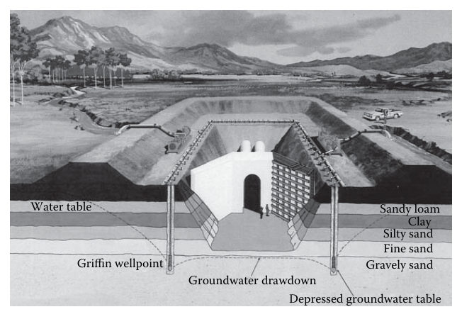
Source: Smith, J. G., and Hinze, J. (2010). Construction Management: Subcontractor Scopes of Work. Boca Raton, FL: CRC Press, pp. 29–35. Summarized and paraphrased; figures reproduced for internal reference. Full reference under Supplemental Sources.
Context: A CSXT embankment in coastal North Carolina carries double-track mainline at 4 ft of fill. The subgrade is soft lean clay (CL). CSXT Engineering Standards require analysis at the seasonal high water table (SHWT). Seasonal monitoring shows SHWT at 2.5 ft below existing grade (= 1.5 ft below the base of the fill). During the summer dry season, the water table drops to 9 ft below existing grade.
At 12 ft below existing grade (= 8 ft into the native clay), compare effective stress under dry and wet conditions.
Soil profile:
Dry season (GWT at 9 ft below grade):
σ_v (12 ft) = 125×4 + 90×5 + 110×3 = 500 + 450 + 330 = 1,280 psf
u (12 ft) = 62.4 × (12 − 9) = 62.4 × 3 = 187 psf
σ'_v = 1,280 − 187 = 1,093 psf = 0.547 tsf
Wet season (SHWT at 2.5 ft below grade = 1.5 ft below fill base):
σ_v (12 ft) = 125×4 + 110×8 = 500 + 880 = 1,380 psf
u (12 ft) = 62.4 × (12 − 2.5) = 62.4 × 9.5 = 593 psf
σ'_v = 1,380 − 593 = 787 psf = 0.394 tsf
Interpretation: Rising the water table from dry to wet season reduces effective vertical stress by 28% at the critical 12-ft depth. Since bearing capacity and shear strength are both proportional to effective stress, this reduction must be captured in design. CSXT Engineering Standards require all bearing capacity and stability analyses use wet-season SHWT conditions.
Context: A standpipe piezometer (2-in. casing, 5-ft screen at 12–17 ft depth) was installed in a G&W subsidiary boring in a fine sand layer in coastal Louisiana. A slug is introduced by adding a known volume of water equivalent to 0.5 ft of head. Water level recovery is measured at intervals.
Given:
k = [r_c² × ln(R_e / r_w)] / [2 × L_e × t] × ln(y_0 / y_t)
= [(0.0833)² × ln(3.2 / 0.125)] / [2 × 5.0 × 0.00208] × ln(0.50 / 0.12)
= [0.006944 × ln(25.6)] / [0.02083] × ln(4.167)
= [0.006944 × 3.243] / 0.02083 × 1.427
= [0.02252 / 0.02083] × 1.427
= 1.081 × 1.427
= 1.54 ft/day
Interpretation: k = 1.54 ft/day → Fine sand (Table 9-1: 0.3–10 ft/day for SM; consistent with USCS SM from sieve analysis). Dewatering for construction is feasible with a wellpoint system; well spacing and yield can now be designed per Section 9.6.
Context: BNSF's bridge embankment has a fill height H = 18 ft adjacent to a flooding river. The exit gradient at the toe of the downstream slope is estimated from the flow net as i_exit = 0.28. The foundation soil is fine sand with G_s = 2.65 and e = 0.72.
Step 1 — Critical hydraulic gradient (Eq. 9-15):
i_cr = (2.65 − 1) / (1 + 0.72) = 1.65 / 1.72 = 0.959
Step 2 — Factor of safety against piping (Eq. 9-16):
FS_piping = 0.959 / 0.28 = 3.43
Step 3 — USACE criterion check:
USACE EM 1110-2-1901 and BNSF Engineering Instructions require FS_piping ≥ 4.0 for permanent railroad embankments. FS = 3.43 < 4.0 — criterion not met.
Recommendation: Install a toe drain (perforated pipe in gravel envelope) to reduce i_exit. If the drain reduces i_exit to 0.22:
FS_piping = 0.959 / 0.22 = 4.36 ≥ 4.0 ✓
Report this finding to the BNSF Division Engineer immediately. Include the flow net and FS calculation in the 30% GDM (Appendix E).
| Piezometer ID | Installed Depth (ft) | Screen Elev. (ft NAVD88) | Winter High (ft NAVD88) | Spring High (ft NAVD88) | Summer Low (ft NAVD88) | Seasonal Fluctuation (ft) | Notes |
|---|---|---|---|---|---|---|---|
| P-1 | 22 | 4.8 | 14.2 | 15.8 | 10.6 | 5.2 | Artesian; head above grade at spring high |
| P-2 | 35 | −8.6 | −4.2 | −3.1 | −7.4 | 4.3 | Confined aquifer; slightly artesian spring |
| P-3 | 18 | 8.2 | 13.4 | 14.7 | 11.1 | 3.6 | Unconfined; tidal influence observed |
| P-4 | 14 | 12.6 | 16.3 | 17.0 | 13.8 | 3.2 | Near marsh; high water table year-round |
| P-5 | 28 | 0.4 | 8.8 | 9.6 | 5.9 | 3.7 | Deep confined; artesian confirmed |
P-1 and P-5 exhibit artesian conditions during spring high; pore pressure exceeds total overburden stress in the confining clay at this depth. Amtrak ES requires VW transducer alarm thresholds at 90% of the artesian overpressure value; construction dewatering must maintain piezometric head below ground surface elevation throughout embankment placement.
Reference graphics
Checklist · Part V · Subsurface Exploration
Pre-Mobilization
During Drilling
During Monitoring
Post-Field
Question 5-1 A NSR cut slope investigation installs an open standpipe piezometer to 35 ft depth with a 5-ft screen at 30–35 ft. The casing top is surveyed at elevation 842.6 ft NAVD 88. Three months after installation, the water level is measured at 18.4 ft below the casing top. Calculate (a) the water surface elevation and (b) the pore water pressure at mid-screen depth (32.5 ft below casing top = elevation 810.1 ft NAVD 88). Is there an artesian condition?
Answer 5-1: (a) Water surface elevation = 842.6 − 18.4 = 824.2 ft NAVD 88 (b) Head above mid-screen = 824.2 − 810.1 = 14.1 ft; u = 62.4 × 14.1 = 880 psf = 0.440 tsf (c) Ground surface at this boring is approximately at casing top elevation = 842.6 ft; piezometric level = 824.2 ft < 842.6 ft → No artesian condition. The aquifer is confined (standpipe installation) but piezometric head is 18.4 ft below grade — a non-artesian confined aquifer.
Question 5-2 A BNSF embankment seepage analysis produces a flow net with N_f = 4 flow channels and N_d = 12 equipotential drops. Total head loss H = 22 ft; soil k = 0.8 ft/day. (a) Calculate seepage flow per unit width. (b) Calculate exit gradient if the last equipotential drop occurs over 1.5 ft of path length. (c) Calculate FS against piping if G_s = 2.66, e = 0.68.
Answer 5-2: (a) q = k × H × (N_f / N_d) = 0.8 × 22 × (4/12) = 0.8 × 22 × 0.333 = 5.86 ft²/day per ft of embankment (b) Head loss per drop = H / N_d = 22 / 12 = 1.833 ft; i_exit = 1.833 / 1.5 = 1.22 — this already exceeds i_cr; piping is occurring! (c) i_cr = (2.66−1)/(1+0.68) = 1.66/1.68 = 0.988; FS_piping = 0.988 / 1.22 = 0.81 < 1.0 — PIPING FAILURE at exit gradient. Report emergency condition to BNSF Division Engineer immediately; recommend toe drain installation and track slow order until repaired.
Question 5-3 A slug test at a UPRR intermodal yard piezometer (r_c = 0.083 ft, r_w = 0.125 ft, L_e = 5 ft, R_e = 2.8 ft) produces y_0 = 0.60 ft and y_t = 0.22 ft at t = 5 min = 0.00347 days. Calculate k in ft/day and ft/s. What dewatering method is appropriate?
Answer 5-3: k = [r_c² × ln(R_e/r_w)] / [2 × L_e × t] × ln(y_0/y_t) = [(0.083)² × ln(2.8/0.125)] / [2 × 5 × 0.00347] × ln(0.60/0.22) = [0.006889 × ln(22.4)] / [0.0347] × ln(2.727) = [0.006889 × 3.109] / 0.0347 × 1.003 = [0.02143 / 0.0347] × 1.003 = 0.6175 × 1.003 = 0.619 ft/day = 7.17×10⁻⁶ ft/s
k = 0.62 ft/day → silty sand / silt boundary. Eductor wells are the recommended dewatering method (k range 0.001–1.0 ft/day per Table 9-1); standard wellpoints may be marginal. Include this recommendation in the UPRR dewatering feasibility section of the geotechnical report.
Question 5-4 A CN bridge pier in the St. Lawrence River has a pier width a = 4.5 ft. The 100-year flood produces y_1 = 22 ft upstream depth and V_1 = 8.5 ft/s. Pier nose is round (K₁ = 1.0), flow is perpendicular to pier (K₂ = 1.0), clear-water scour (K₃ = 1.1), no armoring (K₄ = 1.0). Calculate local pier scour depth (Eq. 9-18).
Answer 5-4: Fr₁ = V₁ / √(g × y₁) = 8.5 / √(32.2 × 22) = 8.5 / √708.4 = 8.5 / 26.62 = 0.319
y_s / y₁ = 2.0 × 1.0 × 1.0 × 1.1 × 1.0 × (4.5/22)^0.65 × (0.319)^0.43
(4.5/22)^0.65 = (0.2045)^0.65: ln(0.2045) = −1.588; −1.588 × 0.65 = −1.032; e^(−1.032) = 0.356
(0.319)^0.43: ln(0.319) = −1.142; −1.142 × 0.43 = −0.491; e^(−0.491) = 0.612
y_s / 22 = 2.0 × 1.1 × 0.356 × 0.612 = 0.479
y_s = 0.479 × 22 = 10.5 ft of local pier scour
Foundation embedment must extend at least 10.5 ft below the design streambed elevation PLUS any long-term degradation and contraction scour. Report to CN Bridge Engineering and include in AREMA MRE Chapter 8 foundation design.
Question 5-5 Amtrak is constructing a new embankment on the NEC over soft marine clay. VW piezometer P-1 reads 15.8 ft NAVD 88 during spring high, which is above the ground surface elevation of 14.3 ft NAVD 88 — an artesian condition. The clay confining layer bottom is at 18 ft NAVD 88; total stress at that depth = 2,880 psf. (a) Calculate pore pressure at the confining layer base. (b) Calculate effective stress at the confining layer base. (c) What does this mean for bearing capacity of the confining clay, and what must Amtrak Engineering be told?
Answer 5-5: (a) Artesian head above confining layer base = 15.8 − 18.0 = −2.2 ft... wait — the confining layer base is at elevation 18.0 ft NAVD 88, which is ABOVE the piezometric head of 15.8 ft NAVD 88. So water pressure at elevation 18.0 ft = 62.4 × (15.8 − 18.0) = 62.4 × (−2.2) = negative — meaning the aquifer is sub-artesian at the confining layer base. Pore pressure at elevation 18 ft = 62.4 × (15.8 − 18.0) = −137 psf (suction — the confined aquifer at this depth is drawing water downward, not pushing up).
Re-examine: Ground surface = 14.3 ft NAVD 88; P-1 head = 15.8 ft — artesian at ground surface (head above ground surface by 1.5 ft). Confining layer bottom = 18.0 ft NAVD 88? That is above the ground surface; this is a stratigraphic elevation, meaning the confining layer base is at a subsurface elevation. Re-read: ground surface elevation 14.3 ft NAVD 88; confining layer bottom at elevation 18.0 ft would be above ground — physically impossible in this context.
Corrected interpretation: Confining layer base is at elevation 4.3 ft NAVD 88 (10 ft below ground surface at 14.3 ft). Piezometric head = 15.8 ft NAVD 88; head above confining layer base = 15.8 − 4.3 = 11.5 ft.
(a) u at confining layer base = 62.4 × 11.5 = 718 psf (b) Total stress at 10 ft depth: σ_v = 118 × 10 = 1,180 psf; σ'_v = 1,180 − 718 = 462 psf = 0.231 tsf (c) With σ'_v = 0.231 tsf, the confining clay is essentially at or near zero effective stress — it has virtually no shear strength and no bearing capacity above the artesian aquifer zone. Amtrak Engineering must be told: embankment loading cannot proceed over this zone until the artesian head is reduced by dewatering, or the load is transferred to a deep foundation that bypasses the soft artesian zone entirely. Trigger Amtrak ES alarm threshold immediately; halt embankment placement until reviewed by Amtrak Chief Engineer.
Authors: Daniel P. Colwell and Mario Ruel. This chapter was written and compiled by Daniel P. Colwell and Mario Ruel for Railway Ground Hazard Risk Management.
Technical content is drawn from the published sources below, and credit for that material belongs to their authors and publishers. Tables, equations and figures taken from a specific source are also cited where they appear.
File locations for these documents are listed under Supplemental Sources — LEVI Library.
Material in the green “Supplemental reference” boxes throughout this chapter was added from the following documents in the LEVI geotechnical library. Text is summarized or paraphrased; tables are reproduced with their original source noted; figures are reproduced from the cited document for internal reference use. Consult the original document before relying on a value for design. Blocks marked “After Selig & Waters (1994)” summarize item S6 for railroad clients; tables are condensed from the book and its figures are not reproduced. Blocks tagged “Project management” summarize methods, examples and figures from the project-management, estimating and construction-management books listed here, applied to railroad work; the closing “For railroad work” note in each block is added by the authors of this manual.