
Geotechnical engineering libraryContact
Geotechnical Services Manual for Railroad Clients
A Consultant's Reference for Delivering Geotechnical Engineering Services Across North American Railroad Capital Programs
Apps on dirtbert.com that support this chapter. Each one runs in a web browser on a desktop or a phone, with nothing to install. How to use the apps (I.3).
NANCY pages ask you to accept the Use and Disclaimers once in each browser.
Retaining structures are among the most consequential geotechnical elements in railroad capital programs. They support embankments, protect cut slopes, carry track surcharge loads, and define the geometric boundary of right-of-way through urban corridors, bridge approaches, and intermodal facilities. Failures are costly, disruptive, and — given the dynamic loading environment of heavy-haul freight — potentially catastrophic.
This chapter presents the geotechnical design framework for retaining structures in railroad service, organized around the requirements of all nine client railroads — CSXT, NSR, G&W, UPRR, BNSF, CPKC, Amtrak, and CN — and grounded in AREMA Manual for Railway Engineering (MRE) Chapter 8 retaining structure provisions and USACE EM 1110-1-1804. We address lateral earth pressure theory (Rankine, Coulomb, at-rest), surcharge loading from Cooper E-80 trains, wall type selection, global stability, drainage, seismic earth pressure by the Mononobe-Okabe method, and client-specific deliverable requirements. All equations are expressed in English units.
Railroad retaining walls differ from highway walls in three important ways:
AREMA MRE Chapter 8, Section 8.3 provides the governing design basis for railroad retaining walls. CSXT Engineering Standards Section 4 and NSR Engineering Standards Manual Section 5 both require AREMA Chapter 8 compliance as a minimum, with client-specific modifications noted in their respective project-specific technical instructions. UPRR and BNSF Engineering Instructions require submittal of wall design calculations signed and sealed by a licensed Professional Engineer in the project state. CPKC Track Standards require metric-system design checks to be converted and verified against English-unit submittals when delivering in the United States. Amtrak Engineering Standards require a seismic design check for all walls in ASCE 7-22 SDC C or higher. CN Engineering Standards require frost penetration checks for all walls in Canadian territory.
For walls that cannot deflect (rigid basement walls, integral abutments, braced excavations), the at-rest coefficient is used:
K₀ = 1 − sin φ' (normally consolidated soils) [Jaky, 1944]
For overconsolidated soils:
K₀(OC) = K₀(NC) × OCR^(sin φ')
The at-rest horizontal earth pressure at depth z is:
σ_h0 = K₀ × γ × z (psf)
where:
Rankine theory assumes a smooth, vertical wall with a horizontal backfill surface. It is the most commonly applied method for preliminary design and is required by AREMA Chapter 8 as a minimum for walls ≤ 20 ft retained height.
K_A = tan²(45° − φ'/2)
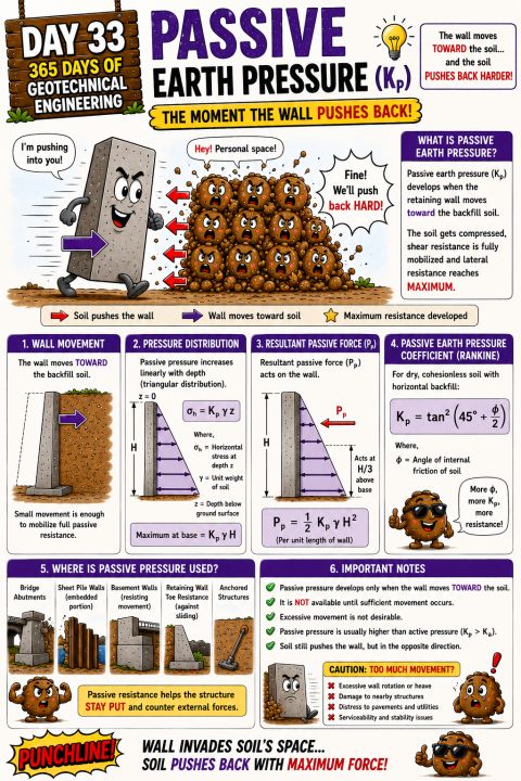
K_P = tan²(45° + φ'/2)
Active pressure at depth z:
σ_A = K_A × γ × z − 2c' × √K_A (psf)
Passive pressure at depth z:
σ_P = K_P × γ × z + 2c' × √K_P (psf)
For purely cohesionless backfill (c' = 0, the standard AREMA design assumption):
σ_A = K_A × γ × z
σ_P = K_P × γ × z
Total active force per linear foot of wall (triangular distribution):
P_A = ½ × K_A × γ × H² (lb/ft)
Acting at H/3 above the base for triangular pressure distribution.
Reference graphics
Coulomb theory accounts for wall friction (δ) and backfill slope angle (β). It is required by AREMA Chapter 8 for walls retaining sloped backfills and for battered walls:
K_A(Coulomb) = sin²(α + φ') / { sin²α × sin(α − δ) × [1 + √( sin(φ' + δ) × sin(φ' − β) / (sin(α − δ) × sin(α + β)) )]² }
where:
For the common case of a vertical wall (α = 90°) retaining horizontal fill (β = 0°):
K_A(Coulomb) = cos²φ' / { cos δ × [1 + √(sin(φ' + δ) × sin φ' / cos δ)]² }
Note: Coulomb passive pressure is non-conservative for walls with significant wall friction; use Rankine passive or log-spiral methods for passive resistance calculations.
In cohesive soils, tension cracking reduces the effective retained height. The tension crack depth is:
z_c = 2c' / (γ × √K_A) (ft)
For design, assume the tension crack is filled with water (worst case). The net active pressure diagram excludes the tension zone, and an additional hydrostatic pressure acts over depth z_c.
AREMA MRE Chapter 8 allows train live load to be represented as an equivalent uniform surcharge on top of the retained fill for wall design:
q_LL = Cooper E-80 wheel load equivalent uniform pressure (psf)
For preliminary design, AREMA Chapter 8 permits the use of:
q_LL = 400 psf (equivalent uniform surcharge for Cooper E-80, per AREMA Ch. 8 commentary)
This is multiplied by DLF = 1.3 (typical Class I value) for dynamic effects, giving a design surcharge:
q_design = DLF × q_LL = 1.3 × 400 = 520 psf
The additional horizontal pressure from this surcharge using Rankine:
Δσ_A(surcharge) = K_A × q_design (psf, uniform with depth)
The resultant surcharge force per foot of wall:
ΔP_surcharge = K_A × q_design × H (lb/ft)
Acting at H/2 above the base (uniform pressure diagram).
For walls within 15 ft of the track centerline (measured horizontally), CSXT Engineering Standards Section 4 and BNSF Engineering Instructions require a more detailed Boussinesq-based pressure distribution using the actual axle loads rather than the simplified equivalent surcharge. Amtrak Engineering Standards require the same for any wall supporting or adjacent to mainline NEC track.
Reference graphics
For excavation support next to active track, CSX (Public Projects Manual, 2020) requires shoring to be designed for active earth pressure plus a live-load surcharge of 1,882 psf on a continuous strip 8.5 ft wide, with lateral pressure computed by the strip-load formula in AREMA MRE Chapter 8, Part 20. (1,882 psf equals an 80-kip E-80 axle spread over 5 ft of track length and 8.5 ft of width.) This is more than three times the 400-psf uniform value in Section 16.3 and, as a strip load, it concentrates pressure in the upper part of the wall. Use the owner’s criterion wherever it applies, and treat the 400-psf equivalent as a preliminary-sizing number only.
Other CSX shoring rules: shoring may be omitted only if the excavation stays outside a 1H:1V line from the bottom corner of the tie and the track is on level ground or in a cut on stable soil. Excavating the toe of an embankment carrying track is not allowed without shoring. Full cofferdams (steel sheeting, or soldier piles and lagging, with wales and struts) are preferred; partial cofferdams open on the side away from the track are allowed where conditions dictate.
Source: CSX Transportation (2020). Public Projects Manual, December 2020 (shoring requirements adjacent to track)
Reference graphics
Reference graphics · click to zoom
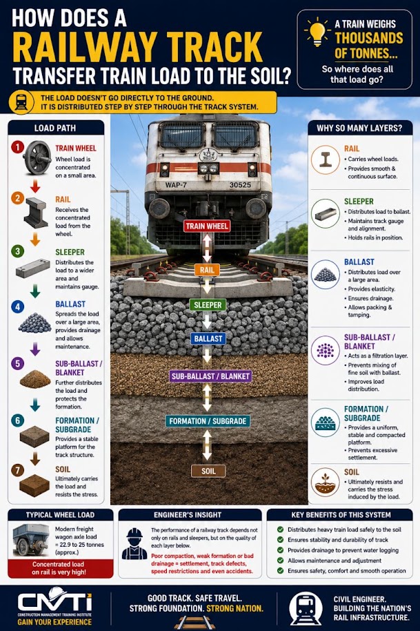
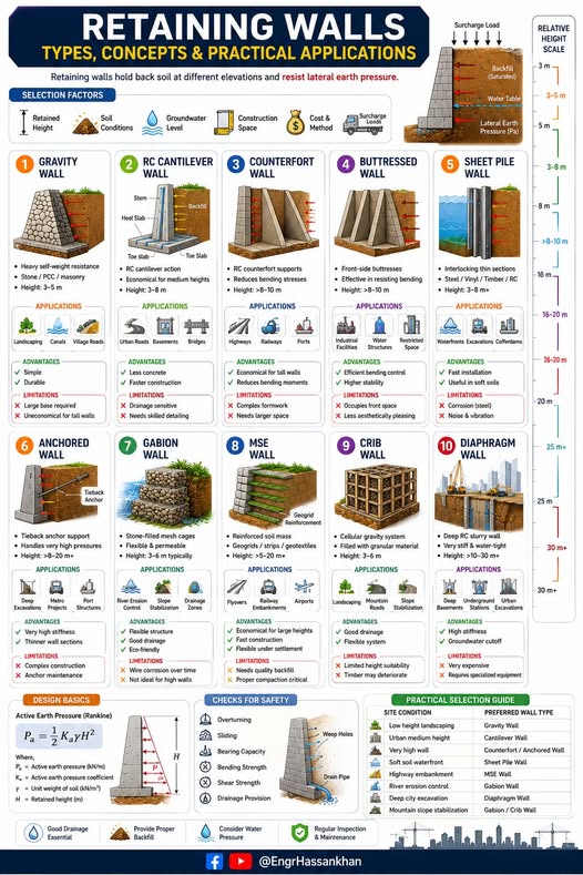
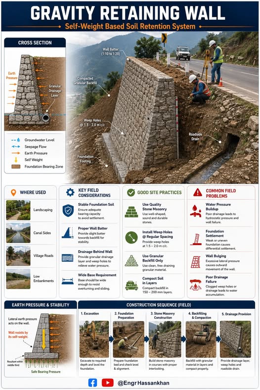
Gravity walls resist sliding and overturning through their own mass. Common materials include mass concrete and dry-laid or mortared stone masonry. Practical retained height limit is approximately 12–15 ft for mass concrete.
Factor of Safety Against Sliding:
FS_sliding = (W × tan δ_base + c_base × B) / P_A_total ≥ 1.5 (AREMA Ch. 8)
where:
Factor of Safety Against Overturning:
FS_OT = ΣM_resisting / ΣM_overturning ≥ 2.0 (AREMA Ch. 8)
Resultant Eccentricity:
e = B/2 − (ΣM_resisting − ΣM_overturning) / ΣV (ft)
For no tension at the base, the middle-third rule requires:
e ≤ B/6
This is a firm requirement under AREMA Chapter 8 and is enforced by all nine client railroads for gravity and cantilever walls supporting track.
Bearing Pressure at Toe:
q_toe = (ΣV/B) × (1 + 6e/B) (psf)
Bearing Pressure at Heel:
q_heel = (ΣV/B) × (1 − 6e/B) (psf)
Reference graphics
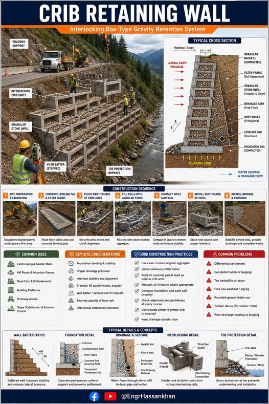
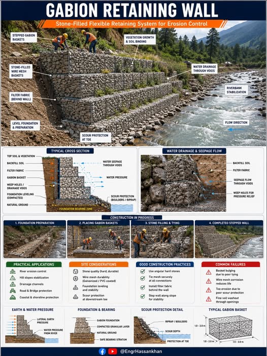
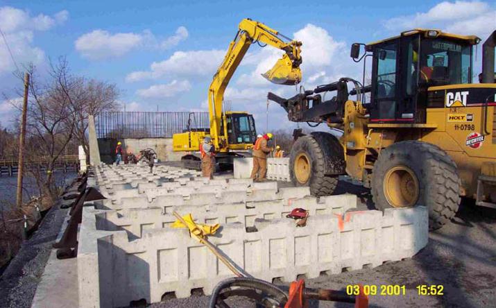
Cantilever walls use a reinforced concrete stem and footing to resist overturning. The critical design section is at the base of the stem. Retained heights of 10–25 ft are typical.
Stem base moment (per foot of wall):
M_stem = (K_A × γ × H³/6) + (K_A × q_design × H²/2) (ft·lb/ft)
Minimum embedment depth for adequate passive resistance:
d_min is determined by setting FS_sliding ≥ 1.5 with the contribution of passive resistance over the embedded depth of the footing toe.
Reference graphics
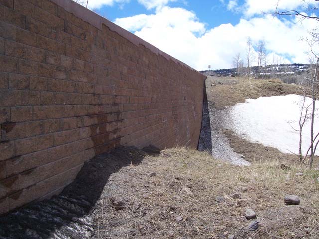
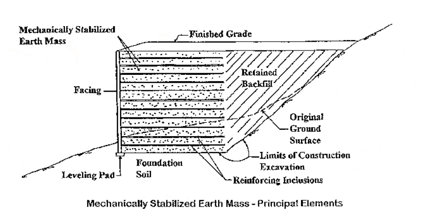
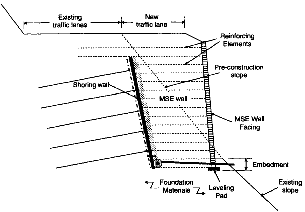
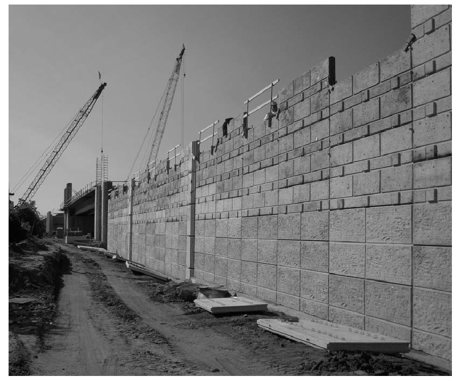
MSE walls use reinforced fill to develop internal stability. They are preferred by UPRR and BNSF for retained heights of 10–40 ft where ROW permits adequate fill width. NSR Engineering Standards Manual Section 5 requires MSE walls to comply with AASHTO LRFD Bridge Design Specifications in addition to AREMA Chapter 8.
Internal stability checks include:
External stability checks (sliding, overturning, bearing) use the MSE mass as an equivalent gravity wall.
AREMA Chapter 8 recommends a minimum 3.5 ft of structural fill (non-MSE) below top of rail elevation for MSE walls adjacent to live track.
Reference graphics
Reference graphics · click to zoom
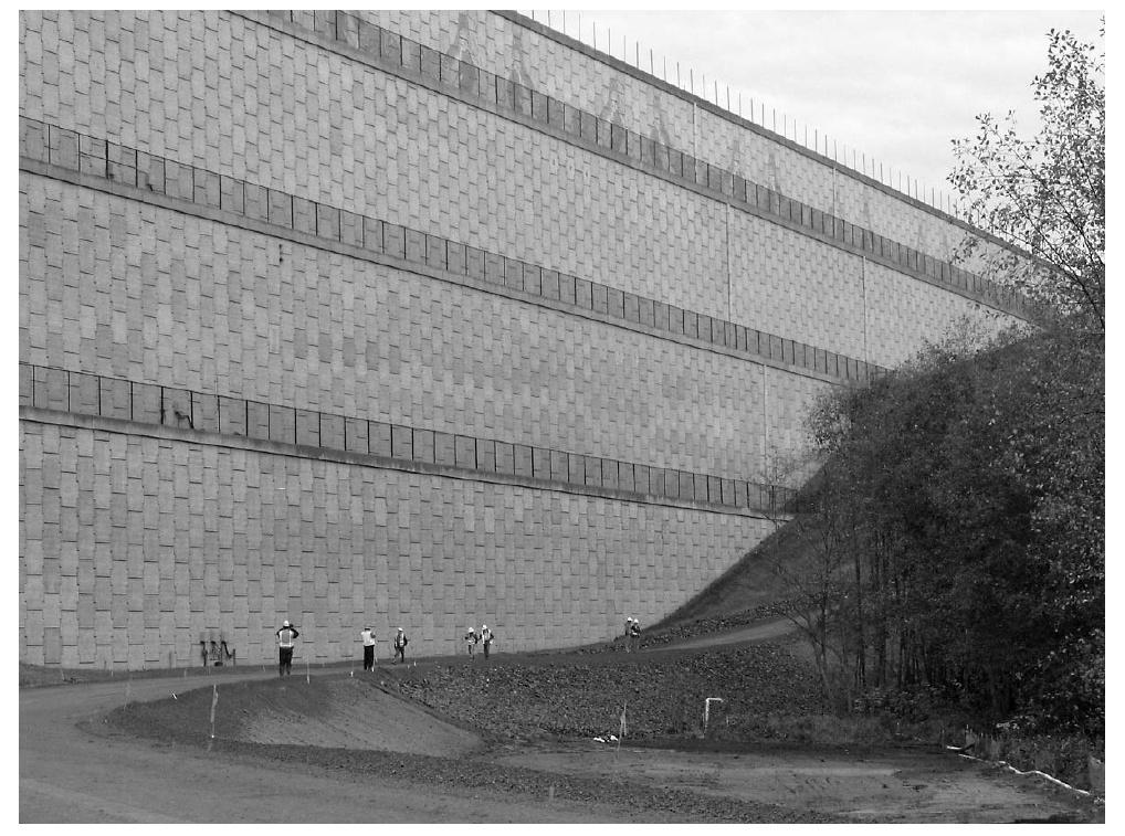
Soldier pile walls use steel H-piles driven or drilled at 6–8 ft spacing with timber lagging. They are commonly used for temporary shoring during cut construction and for permanent retained cuts in urban railroad corridors where MSE fill width is unavailable.
Required embedment depth below excavation for cantilever soldier piles (simplified method):
ΣM_A = 0 → d³ + 1.5H × d² − (P_A × (H + d/3) × 6/K_p × γ) = 0
Solve iteratively for d; increase by factor of 1.2 for design (USACE EM practice).
G&W Engineering Bulletins specify timber lagging thickness as a function of span and soil type; consult the current bulletin for specific G&W projects.
Reference graphics · click to zoom
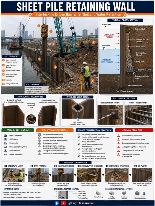
Sheet pile walls (steel) are used for waterfront structures, scour protection, and temporary cofferdams. Free-earth support method for cantilever sheet piles:
d_theoretical is determined by moment equilibrium; design depth = 1.3 × d_theoretical (USACE practice).
Anchored sheet pile walls use tie rods to reduce embedment depth and moment demand. The anchor force:
T_A = P_A − ½ × K_P × γ × d² × (span factor)
CSXT and NSR require coated or encapsulated steel sheet piles for permanent waterfront applications where tidal or chemically aggressive conditions exist.
Reference graphics
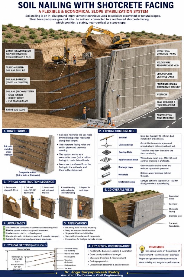
Soil nail walls are constructed top-down and are well suited to cuts in stiff clays, dense sands, and weathered rock. Nail design:
T_design = σ_h × S_v × S_h / FS_nail (lb)
Pullout resistance per unit length: Q_u = π × d_borehole × q_s (lb/ft) where q_s is the unit skin friction (psf)
AREMA Chapter 8 requires a global FS ≥ 1.5 for soil nail walls supporting railroad track.
Reference graphics
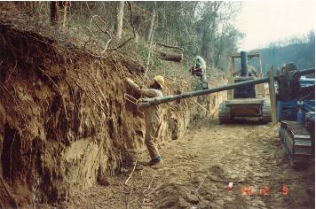
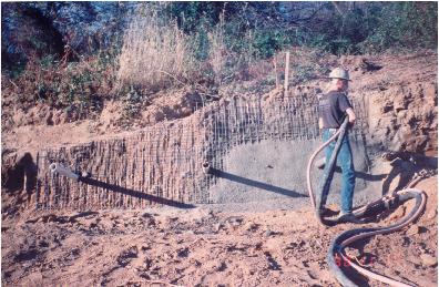
Reference graphics · click to zoom
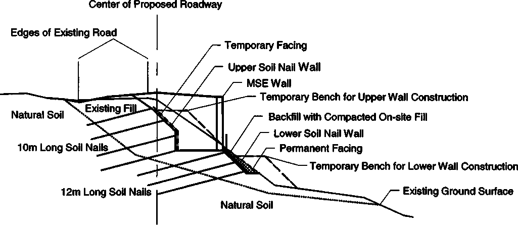
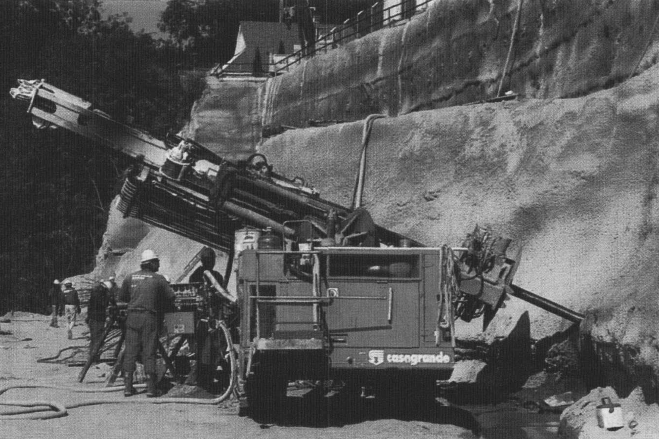
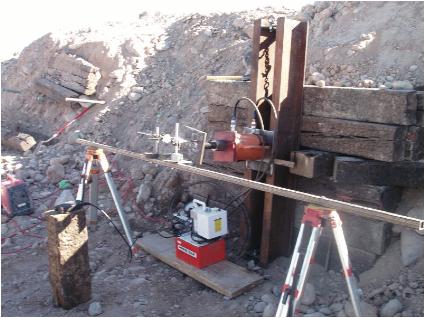
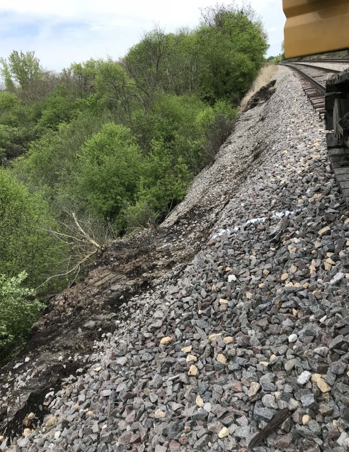
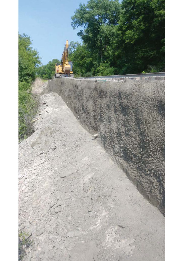
Where a ballast shoulder or fill slope has slumped away from the ties and there is no room or time for a conventional wall, a micropile–tieback facing can be built from the embankment crest within track windows. Two projects in the AREMA Committee 1 files, both by GeoStabilization International (2018), show the arrangement:
Why micropiles fit railroad sites (SHRP2): they can be drilled through any ground, including boulders, rubble fill and old ballast, at any angle, with small rigs, low noise and little spoil (low-headroom rigs work under 10 ft clearance). Capacity comes from grout-to-ground bond (toe resistance neglected), so tension and compression capacities are about equal. At least about 40% of the load is carried by the steel. Capacities commonly exceed 200 tons in soil and 500 tons in rock, and most are under 100 ft long. Limitations: high slenderness (check buckling in very soft or liquefiable soil), and the method depends on contractor drilling and grouting skill, so load testing is essential.
Composite gabion walls (gabion facing combined with tiebacks, soil nails, reinforced concrete beams or drilled shafts) are marketed on the same principle — less excavation behind the face than a gravity gabion or cantilever wall — which matters when the excavation would otherwise undermine the track.
Source: GeoStabilization International (2018). Micropile Tieback Railroad Shoulder Repair, CN Illinois — drawings (Project 180123IL01) and construction photographs. AREMA Committee 1 files · GeoStabilization International (2018). CSX ACCA Yard Culvert Wall — Micropile Cap (drawings). AREMA Committee 1 files · SHRP2 R02 / GeoTechTools (2012). Micro-piles — fact sheet
Section 16.4.5 increases the theoretical embedment by 1.3. EM 1110-2-2504 takes a different approach: it applies a strength-reduction factor to the passive side only (tan φeff = tan φ/FSP; ceff = c/FSP), uses best estimates elsewhere, and usually takes FSA = 1 unless wall deformation must be limited. It then solves directly for the penetration. The two approaches do not give the same depth; do not apply both.
Table 16-S1. Minimum FS on passive pressure for penetration depth (EM 1110-2-2504, Table 5-1, retaining walls)
| Loading case | Fine-grained soils | Free-draining soils |
|---|---|---|
| Usual | 2.00 Q-case; 1.50 S-case | 1.50 S-case |
| Unusual | 1.75 Q-case; 1.25 S-case | 1.25 S-case |
| Extreme | 1.50 Q-case; 1.10 S-case | 1.10 S-case |
Other USACE points relevant to track walls: in medium-dense or denser sand, the active state develops at about 0.4% of wall height (about 1 in. for a 20-ft wall), while full passive needs about 10 times that (about 4%, or 10 in.). This is why passive resistance should be discounted where track settlement is critical. For anchored walls, the Free Earth method gives stable walls with less penetration than Fixed Earth but overpredicts moment (use Rowe’s moment reduction). Initially place the anchor at ¼–⅓ of the exposed height below the top. Grouted anchors must lie entirely outside the active wedge and develop the tie-rod yield strength. Proof-test every anchor to 110% of required resistance and performance-test at least two to 150% of design capacity.
Source: U.S. Army Corps of Engineers (1994). Design of Sheet Pile Walls. EM 1110-2-2504
Lines along coasts, lakes and large rivers often depend on revetments, seawalls or bulkheads. EM 1110-2-1614 sizes armor stone by Hudson’s equation:
W = γrH3 / [KD(γr/γw − 1)3 cot θ]
where W is the armor unit weight (W50 for graded riprap) and H is the design wave height. Suggested KD for breaking waves: rough angular quarrystone, two layers, random 2.0 (1.2 for smooth rounded); graded riprap 2.2 (slopes 2.0–6.0 cot θ). A single layer of randomly placed rough stone is “do not use”, and graded riprap is not recommended where waves exceed 5 ft. For irregular waves on dumped riprap, the zero-damage stability number is Nsz = 1.14 cot1/6 θ with Hs.
Source: U.S. Army Corps of Engineers (1995). Design of Coastal Revetments, Seawalls, and Bulkheads. EM 1110-2-1614
For very tall embankment sides, Profillidis shows either a conventional retaining wall at the toe or reinforced soil: an assembly of good-quality granular backfill, metallic reinforcing bars or strips anchored in the fill, and a concrete facing. Reinforced soil is recommended particularly on poor and very poor subgrades (S1, S0) and allows very steep or vertical faces. A French cost comparison for railway projects found reinforced soil economically and technically advantageous over a retaining wall, especially at heights of 10–40 ft (Figure 16-13).
Caution for electrified lines. The book states that metallic-reinforced soil cannot be used on electrified railways, because return current corrodes the metal reinforcement and can lead to failure. Where a reinforced-soil wall is proposed near an electrified line or a DC transit system, address stray-current corrosion explicitly. Options include non-metallic (geosynthetic) reinforcement or a corrosion design that accounts for stray current.
Figures · click to zoom
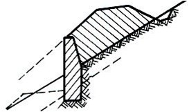
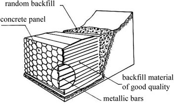
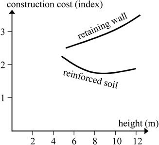
After Profillidis (2014), §9.12.2, §9.13, Figs. 9.16–9.18. Full reference under Supplemental Sources.
Use a wall when a berm cannot be placed. Driven walls isolate the track from shallow-to-medium movement below but are not efficient against deep-seated failures. H-pile walls along the shoulder use piles about 4 ft apart. If movement continues, add a whaler so the piles act together; if it still moves, add soil anchors or tie back to piles on the far side of the grade. Rule of thumb: to hold 4 ft of unstable ground, embed at least 8 ft below the slip plane. At Springhill Mile 84.85, a tidal bank retrogressing toward the track was treated with a temporary riprap toe berm and then a design combining 55-ft H-piles with a 40-ft sheet-pile wall.
Figures · click to zoom
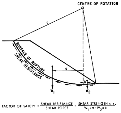
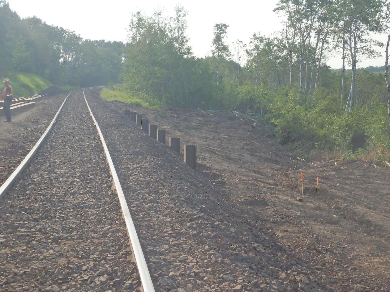
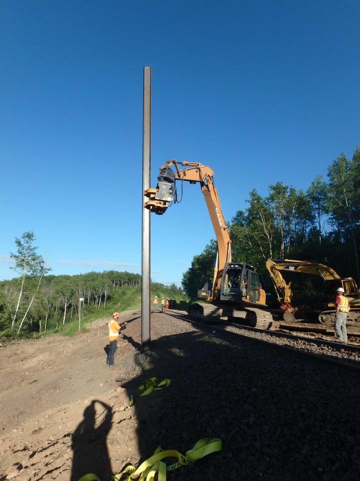
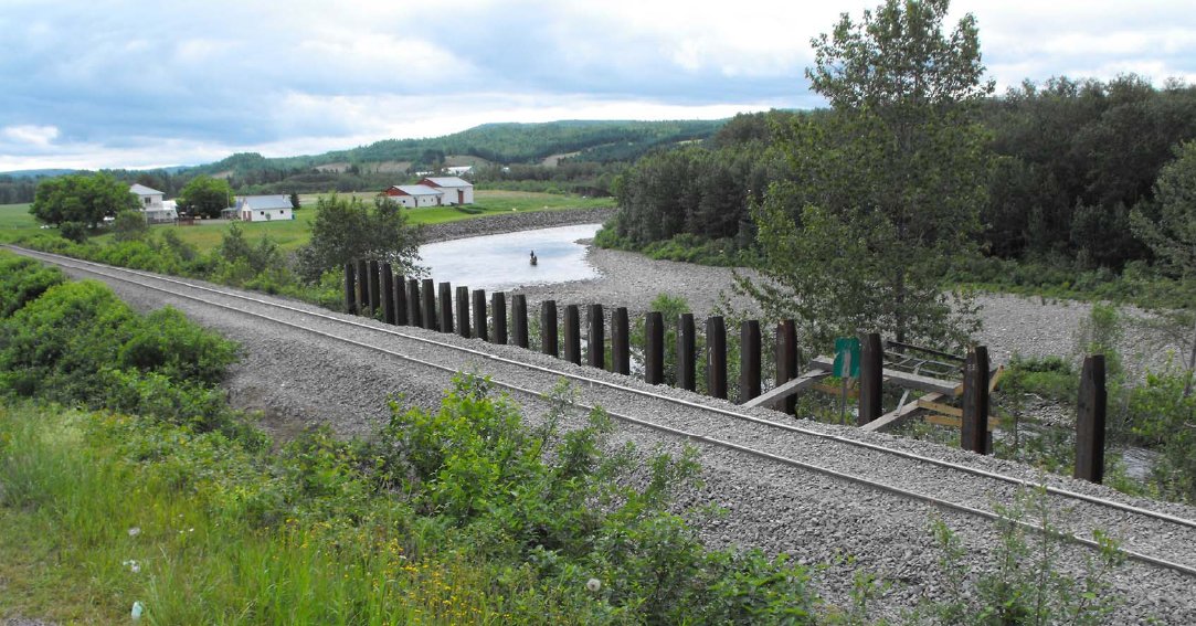
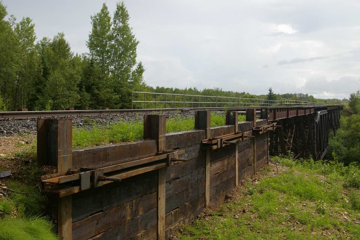
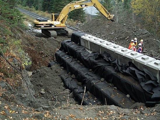
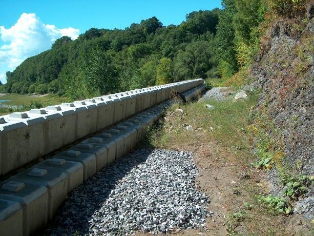
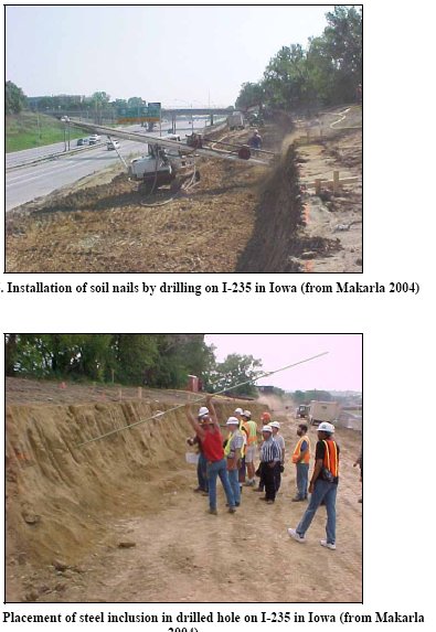
After Geotechnology for Railroaders Program, Module 6.1; §05–07, §10. Full reference under Supplemental Sources.
Cretu et al. argue that risk assessment and value engineering (VE) belong together, because risk analysis characterizes the problems and VE generates the solutions. VE, also called value methodology, is a facilitated multidiscipline study built on function analysis. It asks what an element must do rather than what it is, and that is what separates it from simple cost cutting. For each high or moderate risk they add a function-based step to response planning:
Reducing a long risk narrative to a short function statement keeps the team focused on the thing that can actually be managed. It also tends to produce several candidate solutions instead of one.
For railroad work: Wall selection is a natural application. Suppose the risk is “soft clay below the planned cantilever wall may cause excessive rotation under E-80 surcharge.” The risk object is the foundation. The response functions might be “avoid foundation” (a lightweight-fill embankment or a pile-supported wall), “mitigate settlement” (ground improvement or preloading where a track window allows), “transfer design” (a performance-specified proprietary system) and “accept movement” (a flexible MSE or gabion wall with a resurfacing allowance). Screening these against track-outage limits, construction access from the right-of-way, and the railroad’s preferences for wall type gives a short list. The short list can then be ranked by weighted paired-comparison scoring and compared on a whole-life cost basis.
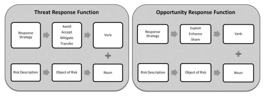
Source: Cretu, O., Stewart, R. and Berends, T. (2011). Risk Management for Design and Construction. Hoboken, NJ: John Wiley & Sons, pp. 157–162. Summarized and paraphrased; figures reproduced for internal reference. Full reference under Supplemental Sources.
Global stability analysis (deep-seated failure of the entire wall-soil system) must be performed for all walls retaining more than 10 ft of fill per AREMA Chapter 8 requirements adopted by all nine client railroads. Use Bishop Simplified (Chapter 13) or Spencer's method for complex geometries.
Minimum global FS values by client (Table 16-1):
| Railroad | Long-Term FS (static) | Seismic FS | Submerged/Seepage FS | Source |
|---|---|---|---|---|
| CSXT | 1.5 | 1.1 | 1.3 | CSXT Eng. Std. Sec. 4 |
| NSR | 1.5 | 1.1 | 1.3 | NSR Eng. Std. Manual Sec. 5 |
| G&W | 1.5 | 1.1 | 1.25 | G&W Eng. Bulletin |
| UPRR | 1.5 | 1.1 | 1.3 | UPRR Eng. Instruction Manual |
| BNSF | 1.5 | 1.1 | 1.3 | BNSF Eng. Instructions |
| CPKC | 1.5 | 1.1 | 1.3 | CPKC Track Standards |
| Amtrak | 1.5 | 1.15 | 1.35 | Amtrak Eng. Std. (higher for pax) |
| CN | 1.5 | 1.1 | 1.3 | CN Eng. Standards |
| AREMA | 1.5 | 1.1 | 1.3 | AREMA MRE Ch. 8 |
Reference graphics
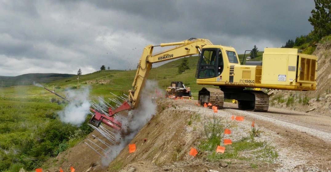
Case study: 16.16.1 Back-analysis of a failed wall: condemn 330 ft, or not? (Look 2023), in §16.16 Case Studies.
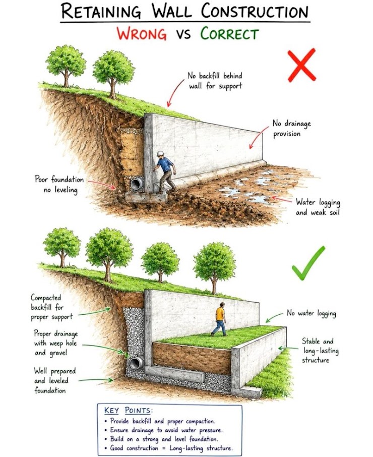
Hydrostatic pressure behind a wall can double or triple total lateral force. Drainage is not optional — it is a fundamental design requirement.
Hydrostatic pressure added to active pressure:
σ_w = γ_w × h_w (psf)
where h_w = height of water behind wall (ft); γ_w = 62.4 pcf.
Design requirement: All walls retaining granular fill must include continuous granular drainage blanket (≥ 12 in. thick, AASHTO No. 57 stone or equivalent), perforated pipe collector drain at the base, and weep holes through the wall face (4 in. diameter minimum, spaced ≤ 10 ft, per AREMA Ch. 8).
For walls in CPKC and CN territory where freeze-thaw cycles are severe, insulated drainage blankets or thermally protected drains are required to prevent pipe freeze.
Reference graphics
A Geosynthetic Research Institute review estimated about 35,000 geosynthetic-reinforced MSE walls, about 30% of them block-faced SRWs. It examined 26 problem walls (12 serviceability, 14 collapses). In 25 of 26 the cause was poor backfill or poor construction and/or lack of inspection, and 20 of 26 had silt or clay backfill in the reinforced zone. The collapse mechanism was hydrostatic pressure: a crack admits water, the facing bulges, a block is dislodged, and the blocks above follow progressively until the facing and drainage gravel are lost.
| Sieve | Koerner (1994) | FHWA (1998) | NCMA (1997) |
|---|---|---|---|
| No. 4 | 100 | 100 | 20–100 |
| No. 40 | 0–60 | 0–60 | 0–60 |
| No. 200 | 0 | 0–15 | 0–35 |
Recommended reinforced-backfill gradations, % passing (GRI compilation).
Recommendations: prefer sand in the reinforced zone (gravel is acceptable but costs more and increases installation damage). If silt or clay is used it must be drained internally and externally, with particular attention to surface drainage. Design for hydrostatic pressure from all sources and directions. Suggested construction QA presence is 67% of construction time for noncritical permanent walls and 100% for critical walls; critical walls next to track should have full-time inspection. The same survey (1998 bid prices from 40 state DOTs) found geosynthetic MSE the least-cost wall type in every height class.
Source: Geosynthetic Research Institute (c. 2000). Geosynthetic Reinforced Segmental Retaining Walls (SRWs) (presentation; cost survey after J. Koerner et al., 1998)
For walls in seismically active zones (ASCE 7-22 SDC B and higher), seismic earth pressure increment must be added to the static active pressure. Amtrak requires seismic design for all mainline NEC walls. UPRR and BNSF require seismic design in SDC C and D zones.
The Mononobe-Okabe (M-O) total active force:
P_AE = ½ × γ × H² × (1 − k_v) × K_AE (lb/ft)
where:
K_AE = cos²(φ' − θ − α) / { cosθ × cos²α × cos(δ + α + θ) × [1 + √(sin(φ' + δ) × sin(φ' − θ − β) / (cos(α + θ + δ) × cos(α − β)))]² }
and:
θ = arctan(k_h / (1 − k_v))
The seismic earth pressure increment:
ΔP_AE = P_AE − P_A (lb/ft)
Per Seed and Whitman (1970), this increment is assumed to act at 0.6H above the base:
M_AE = ΔP_AE × 0.6H + P_A × H/3 (ft·lb/ft)
| Railroad | Min. FS Slide | Min. FS OT | Wall Friction | Surcharge | Seismic Req. | Drain Req. | PE Seal State | Governing Std. |
|---|---|---|---|---|---|---|---|---|
| CSXT | 1.5 | 2.0 | δ = ⅔φ' | 520 psf | SDC C+D | Mandatory | Yes | CSXT Eng. Std. Sec. 4 |
| NSR | 1.5 | 2.0 | δ = ⅔φ' | 520 psf | SDC C+D | Mandatory | Yes | NSR Eng. Std. Sec. 5 |
| G&W | 1.5 | 2.0 | δ = ⅔φ' | 400 psf | SDC D only | Mandatory | Yes | G&W Eng. Bulletin |
| UPRR | 1.5 | 2.0 | δ = ⅔φ' | 520 psf | SDC B+C+D | Mandatory | Yes | UPRR Eng. Instr. Manual |
| BNSF | 1.5 | 2.0 | δ = ⅔φ' | 520 psf | SDC B+C+D | Mandatory | Yes | BNSF Eng. Instructions |
| CPKC | 1.5 | 2.0 | δ = ⅔φ' | 520 psf | SDC C+D | Frost drain | Yes | CPKC Track Standards |
| Amtrak | 1.5 | 2.0 | δ = ⅔φ' | 520 psf | All SDC | Mandatory | Yes | Amtrak Eng. Std. |
| CN | 1.5 | 2.0 | δ = ⅔φ' | 520 psf | SDC C+D | Frost drain | Yes | CN Eng. Standards |
| AREMA | 1.5 | 2.0 | δ = ⅔φ' | 400 psf | SDC per code | Mandatory | Per state | AREMA MRE Ch. 8 |
Project context: NSR Shenandoah Valley Division track extension in western Virginia. A 20-ft retained height cantilever concrete wall is required at a rock cut transition where the natural slope must be cut back to accommodate a second main track. The backfill is compacted granular fill.
Given:
Step 1: Coulomb K_A (vertical wall, horizontal fill, δ = 22.7°)
K_A = cos²(34°) / { cos(22.7°) × [1 + √(sin(34° + 22.7°) × sin(34°) / cos(22.7°))]² }
K_A = (0.829) / { 0.922 × [1 + √(sin(56.7°) × 0.559 / 0.922)]² }
= 0.829 / { 0.922 × [1 + √(0.836 × 0.559 / 0.922)]² }
= 0.829 / { 0.922 × [1 + √0.507]² }
= 0.829 / { 0.922 × [1 + 0.712]² }
= 0.829 / { 0.922 × 2.930 }
= 0.829 / 2.702 = 0.307
Step 2: Active earth pressure resultant (soil only)
P_A(soil) = ½ × K_A × γ × H² = ½ × 0.307 × 120 × (20)² = 7,368 lb/ft
Acting at H/3 = 20/3 = 6.67 ft above base.
Step 3: Active earth pressure resultant (surcharge)
ΔP_surcharge = K_A × q_design × H = 0.307 × 520 × 20 = 3,193 lb/ft
Acting at H/2 = 10.0 ft above base.
Step 4: Total horizontal force
P_total = 7,368 + 3,193 = 10,561 lb/ft
Step 5: Stem base moment
M_stem = P_A(soil) × H/3 + ΔP_surcharge × H/2
= 7,368 × 6.67 + 3,193 × 10.0
= 49,145 + 31,930 = 81,075 ft·lb/ft
This governs the stem reinforcement design (provided to the structural engineer of record).
Step 6: Trial footing geometry — B = 10 ft, footing weight W_f = 1.5 ft deep × 10 ft wide × 150 pcf = 2,250 lb/ft
Estimate W_total = stem + footing + soil on heel ≈ 24,000 lb/ft (from wall geometry; details omitted for brevity).
Step 7: FS_sliding
FS_sliding = W_total × tan(φ'_base) / P_total
= 24,000 × tan(30°) / 10,561 = 24,000 × 0.577 / 10,561 = 1.31
< 1.5 — Not acceptable. Add shear key. With key, passive resistance adds ~4,000 lb/ft:
FS_sliding = (13,848 + 4,000) / 10,561 = 1.69 ✓
Step 8: FS_OT (moments about toe)
ΣM_resist ≈ 24,000 × (10/2 − 1.0) = 24,000 × 4.0 = 96,000 ft·lb/ft (approximate; actual depends on geometry)
ΣM_OT = P_A × H/3 + ΔP × H/2 = 81,075 ft·lb/ft
FS_OT = 96,000 / 81,075 = 1.18
< 2.0 — Revise geometry. Increase base to B = 14 ft; heel extension provides greater restoring moment. After revision:
FS_OT = 142,000 / 81,075 = 1.75 — still marginal; further geometry optimization required.
Practical note: This example illustrates the iterative nature of cantilever wall design. Real-world solutions typically require 3–5 geometry iterations. NSR requires final design calculations to be produced in MathCAD or similar calculation platform and submitted as PDF appendix to the GDR.
Project context: BNSF Kansas City intermodal expansion requires a 30-ft retained height MSE wall along the yard throat to support an approach embankment. Geogrid reinforcement at 2.0-ft vertical spacing.
Given:
Step 1: Maximum tensile force in reinforcement at depth z = 28 ft (second layer from bottom)
σ_h = K_A × γ × z + K_A × q_design
= 0.260 × 125 × 28 + 0.260 × 520
= 910 + 135 = 1,045 psf
T_max = σ_h × S_v × S_h = 1,045 × 2.0 × 1.0 = 2,090 lb/ft
Compare to long-term design strength of geogrid (obtain from product MARV data sheet; typically 3,000–8,000 lb/ft for 30-ft walls). BNSF Engineering Instructions require a minimum 1.5 FS on geogrid MARV strength.
Step 2: Pullout capacity at depth z = 28 ft (embedment length L_e = 4.5 ft beyond failure plane)
F_pullout = f* × α × σ_v' × L_e × R_c × b
where f* = 0.67 tan φ' = 0.67 × tan(36°) = 0.487; α = 0.8 (default); σ_v' = γ × z = 125 × 28 = 3,500 psf; R_c = coverage ratio = 1.0 (full width); b = 1.0 ft
F_pullout = 0.487 × 0.8 × 3,500 × 4.5 × 1.0 × 1.0 = 6,165 lb/ft
FS_pullout = F_pullout / T_max = 6,165 / 2,090 = 2.95 ≥ 1.5 ✓
Step 3: Bearing pressure check
Total vertical load per foot: W = γ × H × L_wall = 125 × 30 × 22 = 82,500 lb/ft (L_wall = 22 ft for 30-ft wall)
Add surcharge: W_q = q_design × L_wall = 520 × 22 = 11,440 lb/ft
ΣV = 93,940 lb/ft
q_bearing = ΣV / L_wall = 93,940 / 22 = 4,270 psf < 6,000 psf ✓
Conclusion: MSE wall with 2.0-ft geogrid spacing is acceptable at this depth. BNSF requires WEAP-verified driven piles if bearing capacity cannot be confirmed by in-situ testing at 4 ft depth.
Project context: UPRR track extension in the Cascades region, Salem OR. A 15-ft gravity wall retains compacted granular fill. Site: SDC D, S_DS = 1.0g, k_h = 0.25, k_v = 0.
Given:
Step 1: K_AE (Mononobe-Okabe)
K_AE = cos²(32° − 14° − 90°) is complex; using simplified Seed-Whitman approximation:
ΔK_AE ≈ (3/4) × k_h = 0.75 × 0.25 = 0.1875
K_AE ≈ K_A + ΔK_AE = 0.307 + 0.188 = 0.495
(Seed & Whitman 1970 simplified; acceptable for φ' = 30–40° and k_h < 0.3)
Step 2: Total seismic active force
P_AE = ½ × K_AE × γ × H² = ½ × 0.495 × 120 × (15)² = 6,683 lb/ft
Static: P_A = ½ × 0.307 × 120 × (15)² = 4,151 lb/ft
Seismic increment: ΔP_AE = 6,683 − 4,151 = 2,532 lb/ft
Step 3: Seismic overturning moment
M_seismic = P_A × H/3 + ΔP_AE × 0.6H
= 4,151 × 5.0 + 2,532 × 9.0
= 20,755 + 22,788 = 43,543 ft·lb/ft
vs. static: M_static = 4,151 × 5.0 = 20,755 ft·lb/ft
Seismic moment is 2.1× the static moment — confirming that seismic design governs wall geometry in SDC D zones. UPRR Engineering Instruction Manual requires that FS_OT ≥ 1.1 under seismic, which the design must satisfy after completing the resisting moment calculation.
| Project | Client | Wall Type | H (ft) | Backfill φ' (°) | K_A | P_A (lb/ft) | q_surcharge (psf) | FS_slide | FS_OT | Seismic |
|---|---|---|---|---|---|---|---|---|---|---|
| Shenandoah Ext. | NSR | Cantilever RC | 20 | 34 | 0.307 | 7,368 | 520 | 1.69* | 1.75* | No |
| KC Intermodal | BNSF | MSE Geogrid | 30 | 36 | 0.260 | 8,775 | 520 | 1.82 | 2.45 | No |
| Cascades Ext. | UPRR | Gravity Conc. | 15 | 32 | 0.307 | 4,151 | 520 | 1.52 | 1.18 seismic | Yes |
| NEC Viaduct | Amtrak | Soldier Pile | 25 | 30 | 0.333 | 7,500 | 520 | N/A | N/A | Yes |
| Prairie Yard | CPKC | MSE Geogrid | 18 | 35 | 0.271 | 4,400 | 400 | 1.92 | 2.60 | No |
| Gulf Coast Ext. | G&W | Cantilever RC | 12 | 28 | 0.361 | 3,114 | 400 | 1.65 | 2.10 | No |
| Western Div. | CN | Gravity Conc. | 10 | 30 | 0.333 | 2,000 | 400 | 1.80 | 2.50 | No |
*After geometry revision with shear key.
Reference graphics
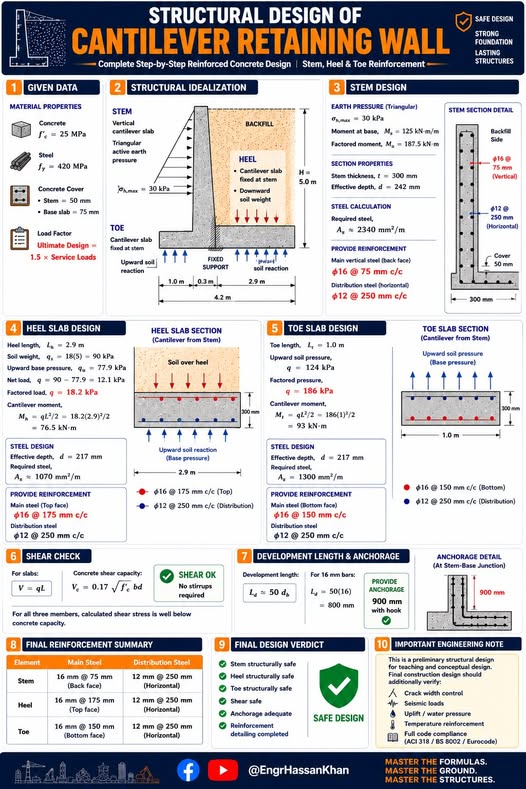

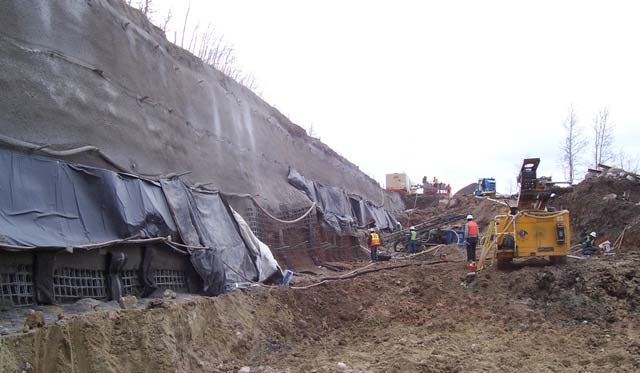
Case study: 16.16.2 Design detailing and analysis input: short case notes (Look 2023), in §16.16 Case Studies.
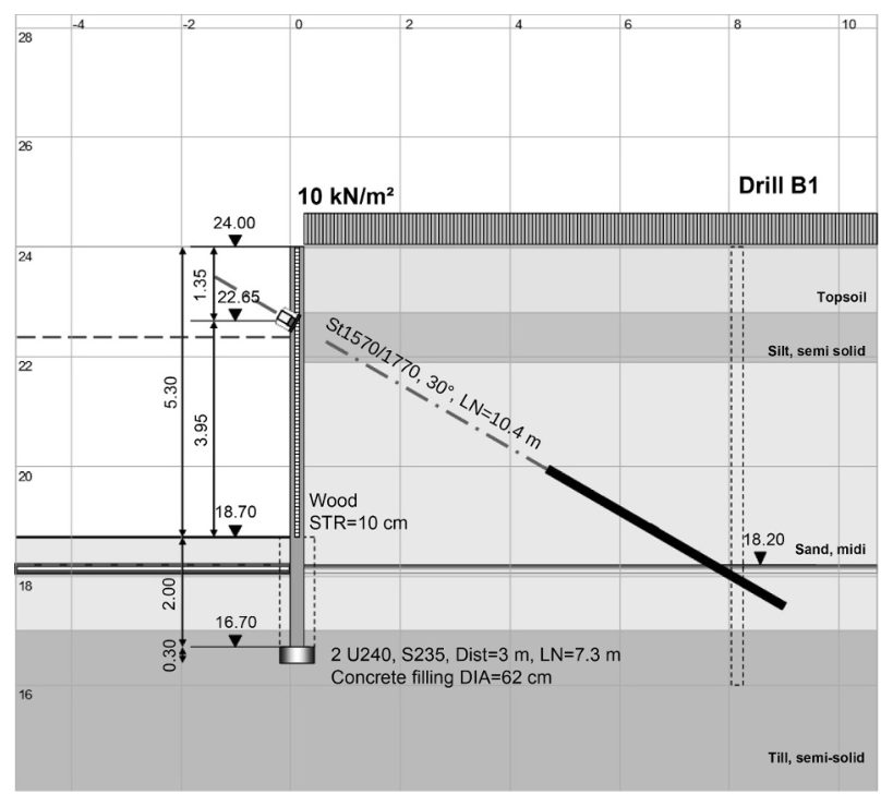
Jacob and Müller price a temporary anchored soldier pile wall by costing one complete bay, meaning one soldier pile and the lagging to the next pile. That bay cost is then spread over the exposed (visible) face area, which is the pay unit in their bill of quantities.
Example geometry, converted to US units:
The bay cost is built from:
Of the bay cost, lagging was about 28%, anchors about 25%, drilling about 25% and extraction about 8%. The bay cost divided by (17.4 ft × 9.8 ft) gives the cost per square foot of face. A 25% markup was applied.
The authors contrast this with sheet piling. Sheet piling is paid on the actual driven wall area rather than the exposed face. When it stays in place permanently, the full material cost is included.
For railroad work: Temporary soldier pile walls for culvert replacements, track-adjacent excavations and shoofly construction are often the largest cost of temporary works. A bay-based build-up shows the railroad how the price depends on several things:
The pay unit (exposed face, total wall area or lump sum) must be stated clearly in the special provision, together with who designs the system and the movement-monitoring limits.
Source: Jacob, D. and Müller, C. (Eds.) (2017). Estimating in Heavy Construction: Roads, Bridges, Tunnels, Foundations. Berlin: Ernst & Sohn, pp. 192–195. Summarized and paraphrased; figures reproduced for internal reference. Full reference under Supplemental Sources.
Checklist · Part VII · Stabilization Methods
Pre-Design Phase
Analysis Phase
Deliverable Phase
| Topic | See Also |
|---|---|
| Bearing capacity of wall foundation | Chapter 11 |
| Settlement of wall foundation | Chapter 12 |
| Global slope stability of retained embankment | Chapter 13 |
| Seismic hazard and k_h determination | Chapter 14 |
| Drainage and seepage behind walls | Chapter 9 |
| Geotechnical Special Provisions (wall language) | Appendix C |
| Retaining wall section in final GDR | Appendix E |
| Foundation soil lab testing | Chapter 10 |
Q1. A vertical cantilever wall retains 18 ft of compacted granular fill (φ' = 32°, γ = 118 pcf). Using Rankine theory, calculate: (a) K_A, (b) total active force P_A per foot of wall from soil only, and (c) additional force from a 520-psf uniform surcharge.
Answer:
Q2. A gravity wall has total resisting vertical load ΣV = 18,000 lb/ft, base width B = 8 ft, and total horizontal active force P_total = 7,200 lb/ft. The eccentricity is e = 1.2 ft. Calculate: (a) FS_sliding (φ'_base = 30°, no key, no adhesion), (b) toe bearing pressure, and (c) check middle-third rule.
Answer:
Q3. A UPRR wall in the Pacific Northwest is in SDC D (k_h = 0.28). The static P_A = 5,500 lb/ft for H = 16 ft. Using the Seed-Whitman simplified approximation, estimate: (a) ΔK_AE, (b) ΔP_AE, and (c) additional seismic overturning moment about the base.
Answer:
Q4. An MSE wall retains 25 ft of fill (γ = 122 pcf, φ' = 35°). At depth z = 22 ft, the geogrid has S_v = 2.0 ft and coverage ratio R_c = 1.0. The pullout embedment length beyond the failure surface is L_e = 5.0 ft, f* = 0.80 tan φ'. (a) Calculate σ_h at z = 22 ft (include 400-psf surcharge). (b) Calculate T_max. (c) Calculate pullout capacity and FS.
Answer:
Q5. Amtrak requires FS_OT ≥ 2.0 for a 22-ft wall under static conditions and FS_OT ≥ 1.15 under seismic conditions. If the static overturning moment is 95,000 ft·lb/ft and the seismic moment (including increment) is 155,000 ft·lb/ft, what minimum resisting moment ΣM_R is required to satisfy both conditions?
Answer:
This is the minimum required resisting moment; the wall geometry (footing width and mass) must be sized to achieve this value. Increasing B from 11 ft to 14 ft typically achieves the necessary moment arm increase for a 22-ft cantilever wall.
Field case studies by Burt G. Look, from Earthworks: Theory to Practice – Design and Construction (CRC Press/Balkema, 2023), chosen for this chapter’s topics. Each is summarized from the book with its key figures and a closing note on railroad application added by the authors of this manual. Credit for the case material belongs to Look; see item S11 under Supplemental Sources.
Related section: 16.5 Global Stability of Retaining Structures
In an extreme 2008 rainfall, 79 ft of a ten-year-old retaining wall, about 6.6 ft high, failed. The client proposed to condemn the remaining 328 ft as well, a replacement of over AU$1 million, because a back-analysis of the failure using saturated soil mechanics, a single-stage failure and a high water table gave the intact wall a factor of safety below 1.2 (Look, 2016).
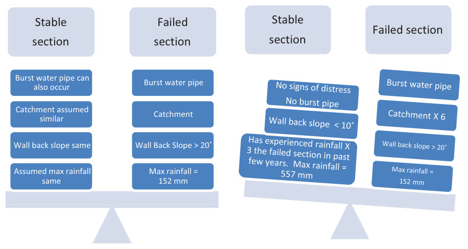
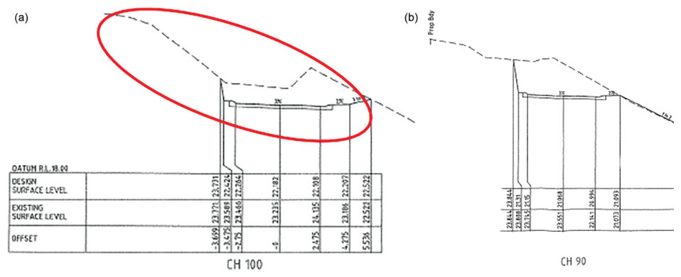
The failed and intact sections were not alike:
No groundwater had ever been seen at this elevated road, and residents reported the failure developed over two days. Coupling finite element seepage with limit equilibrium showed that rainfall reduced soil suction rather than raising a water table. The three back-analyses led to three conclusions for the intact wall:
The intact wall had since come through several large storms with no distress. Look’s lessons: saturated and unsaturated analyses can disagree; back-analysis carries its assumptions into the result; a factor of safety is a decision tool, not an end in itself; and analysis is not design. A slope above a wall can raise active pressure by a factor of three, so the lowest wall is not necessarily the lowest load.
For railroad work: before parameters from a failed retaining wall or cut are applied to the rest of a structure, compare catchment, back slope, water sources and soil depth section by section. Antecedent rainfall, not daily rainfall alone, is the trigger to compare.
Source: Look, B. G. (2023). Earthworks: Theory to Practice – Design and Construction. CRC Press/Balkema. Case study §13.12, pp. 484–490. Summarized and paraphrased; figures reproduced for internal reference. Full reference under Supplemental Sources.
Related section: 16.12 Practical Recommendations
Look closes the design chapter with several short cases where the analysis was right but the detail or the input was not:
For railroad work: side-hill fills are among the most common chronic slide sites on mountain and river-grade lines. When one is rebuilt, the benching or keying detail matters as much as the stability analysis. Surcharge and unloading near buried utilities that cross the right-of-way need their own deflection check.
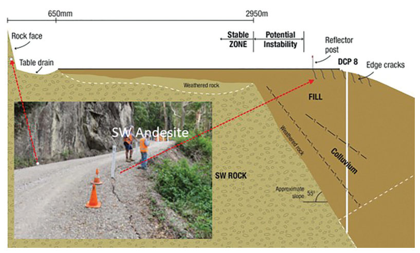
Source: Look, B. G. (2023). Earthworks: Theory to Practice – Design and Construction. CRC Press/Balkema. Case study §13.13, pp. 490–494. Summarized and paraphrased; figures reproduced for internal reference. Full reference under Supplemental Sources.
Authors: Daniel P. Colwell and Mario Ruel. This chapter was written and compiled by Daniel P. Colwell and Mario Ruel for Railway Ground Hazard Risk Management.
Technical content is drawn from the published sources below, and credit for that material belongs to their authors and publishers. Tables, equations and figures taken from a specific source are also cited where they appear.
File locations for these documents are listed under Supplemental Sources — LEVI Library.
Material in the green “Supplemental reference” boxes throughout this chapter was added from the following documents in the LEVI geotechnical library. Text is summarized or paraphrased; tables are reproduced with their original source noted; figures are reproduced from the cited document for internal reference use. Consult the original document before relying on a value for design. The Case Studies section summarizes case studies from item S11 by Burt G. Look; its figures are reproduced from the book for internal reference use, and the closing “For railroad work” note in each case study is added by the authors of this manual. Blocks tagged “Project management” summarize methods, examples and figures from the project-management, estimating and construction-management books listed here, applied to railroad work; the closing “For railroad work” note in each block is added by the authors of this manual.