↑ Parent Menu⌂ Main Menu
← Railway Ground Hazard Risk Management
NANCY
Railway Ground Hazard Risk Management · Part VII · Stabilization Methods
Sections · click a car to open it

Chapter 17 — Ground Improvement Methods

Ground improvement is a fundamental tool in the railroad geotechnical consultant's toolkit, employed when in-situ subgrade conditions cannot support track, structure, or…
Authors: Daniel P. Colwell and Mario Ruel

Primary Reference: USACE EM 1110-1-1804, Geotechnical Investigations (January 2001); FHWA NHI-06-019 "Ground Improvement Methods" (2006); Barron (1948); Priebe (1995); AREMA MRE Chapter 1 (Track Structure and Earthwork); Kirsch & Bell (2012) "Ground Improvement"; ASTM D698 (Standard Proctor); ASTM D1557 (Modified Proctor).

Apps for this Chapter1

Apps on dirtbert.com that support this chapter. Each one runs in a web browser on a desktop or a phone, with nothing to install. How to use the apps (I.3).

NANCY pages ask you to accept the Use and Disclaimers once in each browser.

17.0 Executive Summary

Ground improvement is a fundamental tool in the railroad geotechnical consultant's toolkit, employed when in-situ subgrade conditions cannot support track, structure, or facility loads without unacceptable settlement, slope instability, or bearing capacity failure. Railroad projects present a concentrated set of ground improvement challenges: soft coastal and alluvial clays crossed by CSXT and CN mainlines, expansive Prairie clays along BNSF and CPKC corridors, loose liquefiable sands requiring treatment for UPRR and Amtrak facilities, and organic deposits that underlie historic rail alignments across multiple clients.

This chapter presents methods for: (1) densification by compaction — mechanical, dynamic, and vibratory; (2) consolidation acceleration using prefabricated vertical drains (PVDs) with staged embankment loading; (3) stone column reinforcement with the Priebe method for composite stiffness; (4) deep soil mixing (DSM) for soft clay improvement and liquefaction mitigation; (5) grouting — permeation, compaction, and jet grouting; (6) lime and cement stabilization; and (7) geosynthetic reinforcement for embankment and subgrade applications. All equations are in English units.

17.1 Background and Railroad Context

Railroad ground improvement projects carry constraints not present in highway or building construction:

  • Active operations: Most ground improvement beneath or adjacent to active track must be designed for minimal vibration transmission to avoid track geometry disturbance. Dynamic compaction and heavy drop weights are generally prohibited within 100 ft of active track without client-approved vibration monitoring protocols.
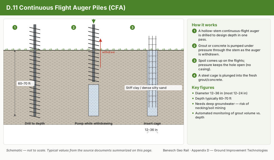
  • Access limitations: Narrow railroad rights-of-way — often 50–100 ft between fence lines — limit crane swing radii, restricting some methods (stone columns, auger-cast piles) to compact equipment configurations.
  • Track geometry tolerance: Post-improvement differential settlement criteria are driven by FRA track class tolerances (Chapters 12 and 18), not building codes. Methods must be designed to achieve residual differential settlement within those limits.
  • Rapid execution: Emergency and programmatic track improvement projects often have compressed schedules. Methods selected must be compatible with railroad-standard maintenance windows (e.g., 4-hour possession on mainline, weekend gang windows on secondary).
Table 17-1: Ground Improvement Method Selection by Railroad Client
RailroadPreferred MethodsProhibited/Restricted MethodsGoverning Standard
UPRRPVDs + surcharge; stone columns; DSM for liquefactionDynamic compaction within 200 ft of trackUPRR EIM — Embankment & Ground Improvement
BNSFPVDs + staged loading; compaction grouting; geosyntheticsVibro-flotation within 150 ft track (unless monitored)BNSF EI — Embankment Design
CSXTPVDs + surcharge; lime/cement; geosyntheticsDynamic compaction within 100 ft trackCSXT ES — Embankment Construction
NSRPVDs; geosynthetics; lime stabilizationVibro-replacement within 100 ft active trackNSR ESM — Earthwork
AmtrakDSM; jet grout; PVDs; rigid inclusionsDynamic compaction prohibited NECAmtrak ES — Ground Improvement
CPKCPVDs + surcharge; cement; geosynthetics; frost protectionDynamic compaction winter operationsCPKC TS — Embankment and Subgrade
CNPVDs; stone columns; DSM; geosyntheticsDynamic compaction within 150 ft trackCN ES — Embankment Design
G&WLime/cement; geosynthetics; compaction groutingPer regional jurisdictionAREMA MRE Chapter 1
AREMAAll methods per site conditionsPer owner approvalAREMA MRE Chapter 1

Reference graphics · click to zoom

Soil Compaction & Ground Improvement Techniques

Improving the formation layer under an existing track

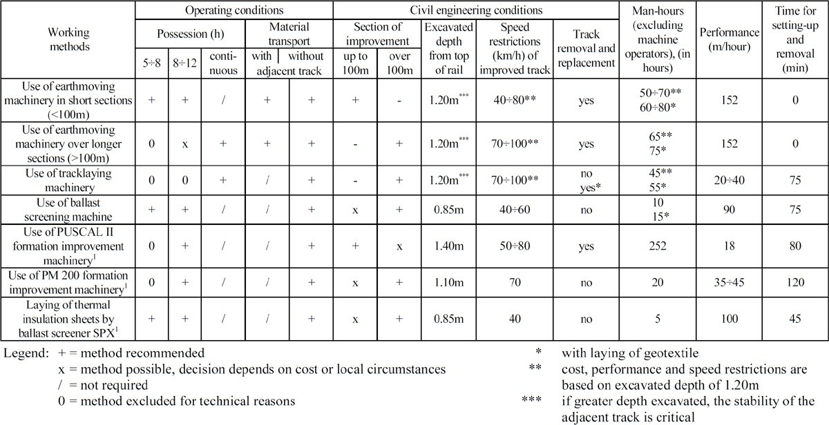
Many old lines were built without a formation layer. When speed or axle load is raised, the simplest fix is to thicken the track bed during maintenance, but clearance limits or stress targets often rule that out, and the formation layer itself must be improved or installed. The UIC methods compiled by Profillidis differ mainly in possession time, excavation depth and output:

Table 17-5. Methods for improving the formation layer under traffic (summary)
MethodExcavation below top of railSpeed on improved track (mph)Track removed?Output (ft/h)
Earthmoving machinery, short sections (< 330 ft)4 ft25–50Yes500
Earthmoving machinery, longer sections (> 330 ft)4 ft43–62Yes500
Track-laying machinery4 ft43–62No (yes with geotextile)66–130
Ballast screening machine33 in.25–37No295
PUSCAL II formation-improvement machine4.6 ft31–50Yes59
PM 200 formation-improvement machine3.6 ft43No115–150
Thermal insulation sheets laid by ballast screener SPX33 in.25No330

Excavating deeper than 4 ft makes the stability of the adjacent track critical. Full table, with possession hours and man-hours, in Figure 17-11.

Formation rehabilitation machines insert a new sand–gravel formation layer at the top of the subgrade without removing the track. They are the substructure equivalent of ballast cleaning, for sites where subgrade bearing capacity, not ballast condition, is the problem.

Figures · click to zoom

Figure 17-11. Methods for improving the formation layer, with possession, transport, depth, speed, man-hour and output data. Profillidis Table 9.4.

After Profillidis (2014), §9.7.2, §16.8, Table 9.4; after UIC Code 722R. Full reference under Supplemental Sources.

Subgrade stabilization categories and costs

Subgrade stabilization follows the same logic as slope work. Rehabilitate drainage first, then reinforce the substructure below the ballast and the track structure above it, and improve the ground itself where the problem runs deep.

Table 17-6. Remedial categories and indicative costs (course figures, 2016 dollars)
CategoryExamplesIndicative cost (2016 $)
Improve structure above trackEliminate joints, heavier rail, swamp tiesSwamp ties ~$670,000/mile [2012: ~$600,000]
Improve substructure below ballastUndercutting / ballast replacement, geogrid, HMA underlaymentUndercutting ~$280,000/mile [2012: ~$250,000]
Improve subgrade strengthShear key, cross trench, cement or grout injection, remove and replaceSite-specific
UnderpinningMicropiles, screw pilesSite-specific
(Reference) new construction~$6,700,000/mile [2012: ~$6,000,000]

Cost basis: The course figures were in 2012 dollars. They are escalated here to 2016 dollars with the ENR Construction Cost Index (20-city annual average): 10,338 (2016) ÷ 9,308 (2012) = 1.111, an increase of about 11%. Values are rounded; 2012 values are shown in brackets. To move to another year, multiply the 2012 value by CCIyear ÷ 9,308. Railroad work (track time, work trains, flagging, remote access) can vary by far more than the index change, so treat these as order-of-magnitude figures.

Figures · click to zoom

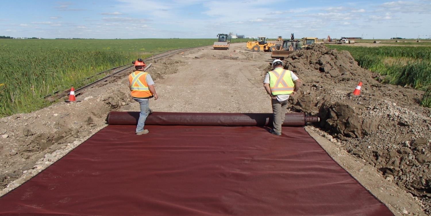
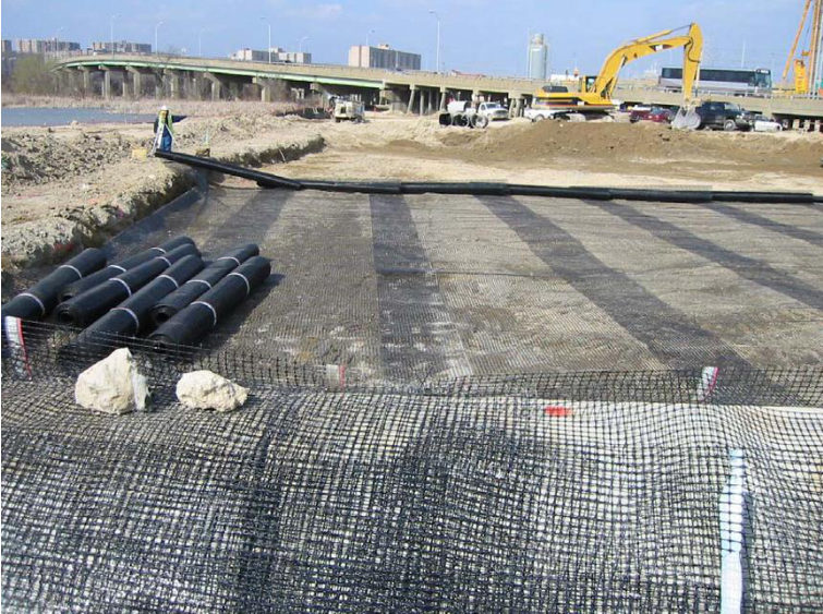
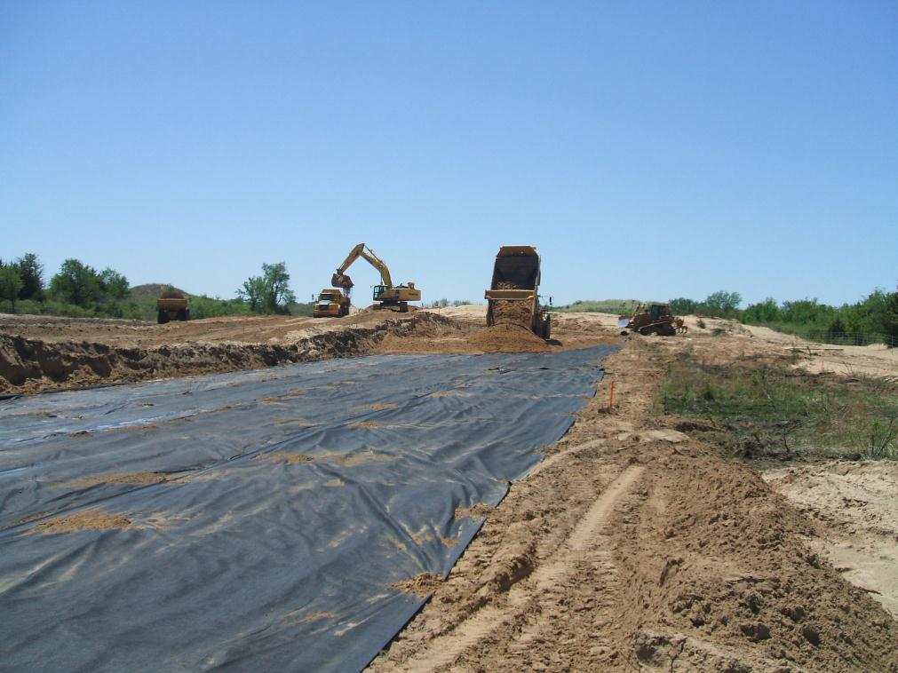
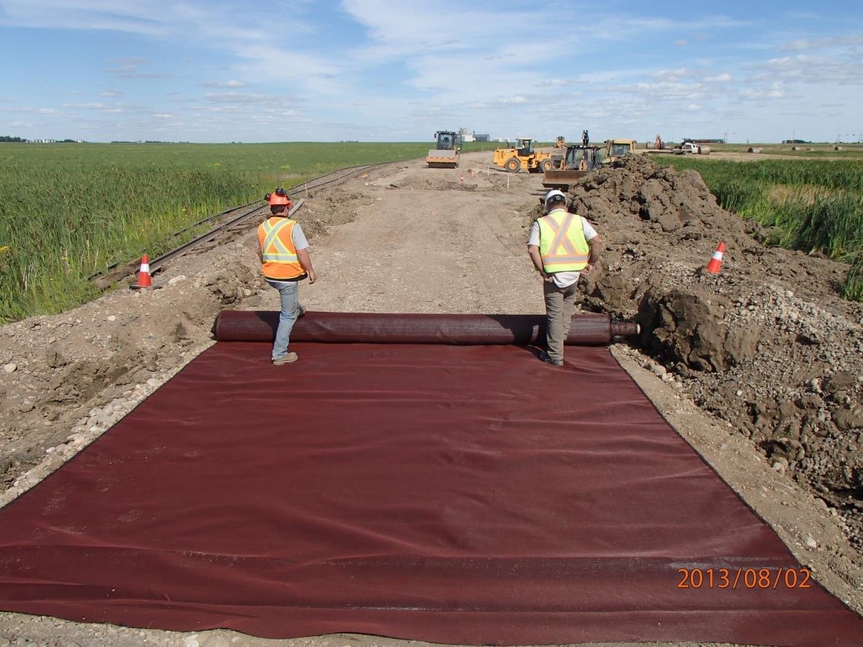
Figure 17-13. Rolling out geotextile ahead of subgrade rebuilding.

After Geotechnology for Railroaders Program, Module 6.2; §01. Full reference under Supplemental Sources.

Improvement options for existing track

Selig and Waters group the options for existing track into four families:

  • In place: penetration or compaction grouting, lime-slurry injection, electro-osmosis and electrochemical treatment.
  • Reconstruction: compaction, replacement, or admixtures of cement, lime, fly ash or bitumen.
  • Asphalt: full depth or underlayment (Section III, §3.8).
  • Slip stabilization: drainage, retaining structures, slope changes.

Notes on the in-place methods.

  • Electro-osmosis and electrochemical stabilization work from beside the track without interrupting traffic, but they are very expensive.
  • Lime-slurry injection (50–250 psi) follows existing fissures, so placement is poorly controlled. Where K0 < 1 the hydrofractures run vertically, and the slurry can escape into the ballast. Results have been mixed and sometimes adverse, with temporary weakening and lime-fouled ballast. Run a full-scale trial before committing.

After Selig & Waters (1994), ch. 11. Full reference under Supplemental Sources.

Project management · Sears et al. (2015)

Choosing the Delivery Method and Pricing Basis

Sears et al. separate two decisions that are often blurred together: how the project is delivered and how the contractor is paid.

Delivery methods.

  • Design-bid-construct. The design is finished before bidding. The owner knows the configuration and cost before committing, but the process is the slowest.
  • Fast-tracking (phased construction). Packages are let as each part of the design is completed. This saves time but adds coordination risk.
  • Design-construct. One firm designs and builds, bringing contractor knowledge of methods, cost and time into the design. It is usually negotiated.
  • Construction management. Agency CM advises the owner and builds nothing. CM-at-risk commits to cost and schedule at an early stage of design.
  • Turnkey and build-operate-transfer. These extend the contractor’s responsibility further, into areas such as financing and operation.

Pricing bases.

  • Lump sum. Suitable only when both the nature and the quantity of the work can be fixed before award.
  • Unit price. Suited to work whose nature is well defined but whose quantities cannot be forecast accurately. The contractor is paid measured quantities at bid rates, subject to any clause allowing rates to be renegotiated for large quantity changes.
  • Cost-plus-fee. The fee is a percentage or a fixed sum, often with incentives or a guaranteed maximum.
  • Force account. The owner does the work with its own forces, or the contractor works under owner direction on time and materials for work that cannot be defined or has changed. Public agencies usually limit force account to maintenance, repair and emergencies.

Selection. The authors also describe best-value selection, which scores price together with qualifications, as increasingly accepted.

For railroad work: Ground improvement is where these choices matter most, because the quantity of ground treated is uncertain and the result is a performance outcome rather than a quantity. Practical pairings to consider:

  • Unit-price contracts for undercutting, blanket placement and grouting, where the method is known but depth and take are not.
  • Design-build with a performance specification for proprietary systems such as deep soil mixing, rigid inclusions or compaction grouting, with acceptance tied to verification testing and settlement monitoring.
  • Force account or time-and-materials for slide emergency response, converting to a defined contract once the failure is mapped.

Whatever the method, the GSPs and the geotechnical report should state which party carries quantity risk and which carries performance risk.

Source: Sears, S. K., Sears, G. A., Clough, R. H., Rounds, J. L., and Segner, R. O., Jr. (2015). Construction Project Management: A Practical Guide to Field Construction Management, 6th ed. Hoboken, NJ: John Wiley & Sons, pp. 6–13. Summarized and paraphrased. Full reference under Supplemental Sources.

17.2 Compaction Methods
17.2.1 Proctor Compaction Fundamentals

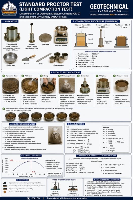
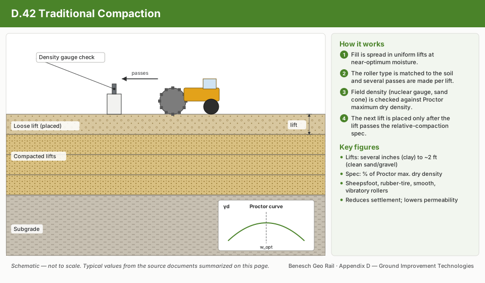
The relationship between dry unit weight and moisture content is defined by the Proctor test. The maximum dry unit weight γ_d,max and optimum moisture content w_opt are the design targets for compaction control (Chapter 15).

Zero Air Voids (ZAV) line:

γZAV = Gs ⋅ γw1 + w ⋅ Gs    (pcf)

Where G_s = specific gravity (≈ 2.70 for most soils); γ_w = 62.4 pcf; w = water content (decimal).

Relative compaction (RC):

RC = γd,fieldγd,max × 100%

Standard Proctor (ASTM D698): 12,400 ft·lb/ft³ compactive effort; appropriate for light to moderate railroad facility construction. Modified Proctor (ASTM D1557): 56,250 ft·lb/ft³ compactive effort; required for intermodal yards, bridge approach fills, and all UPRR, BNSF, CPKC, and CN embankments.

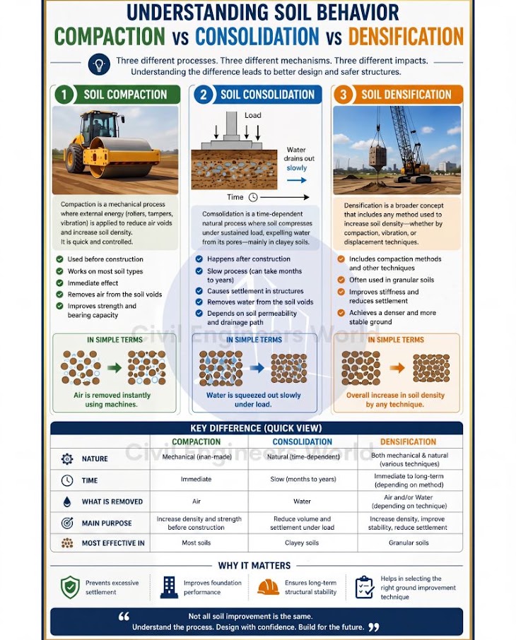
Reference graphics

Understanding Soil Behavior — Compaction
Standard Proctor Test

Reference graphics · click to zoom

Soil Compaction
Soil Compaction
17.2.2 Vibratory Compaction

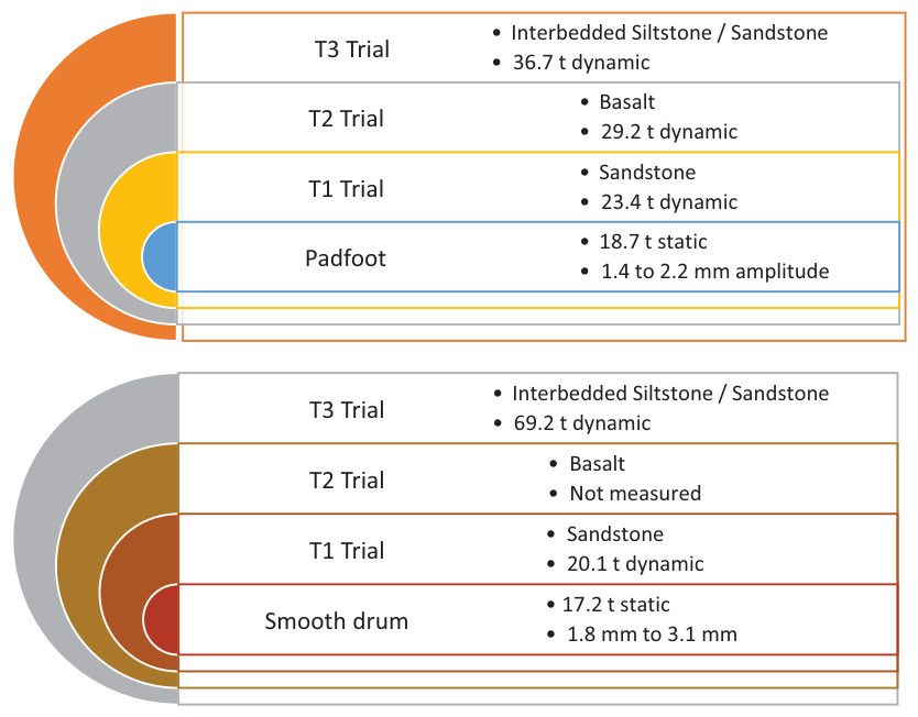
Vibratory compaction (smooth drum, padfoot) densifies granular fills and coarse-grained subgrades. Compaction effectiveness is described by the influence depth Z_eff:

Zeff = k √WAf    (ft)

Where W = drum weight (lb); A_f = drum contact area (ft²); k = empirical constant (0.08–0.12 for granular materials).

Lift thickness limits by soil type:

  • Granular (GW, GP, SW): 12–18 in. uncompacted
  • Silty/clayey soils (SM, SC, ML, CL): 8–12 in. uncompacted
  • Heavy clay (CH): 6–8 in. uncompacted (padfoot drum required)

Reference graphics

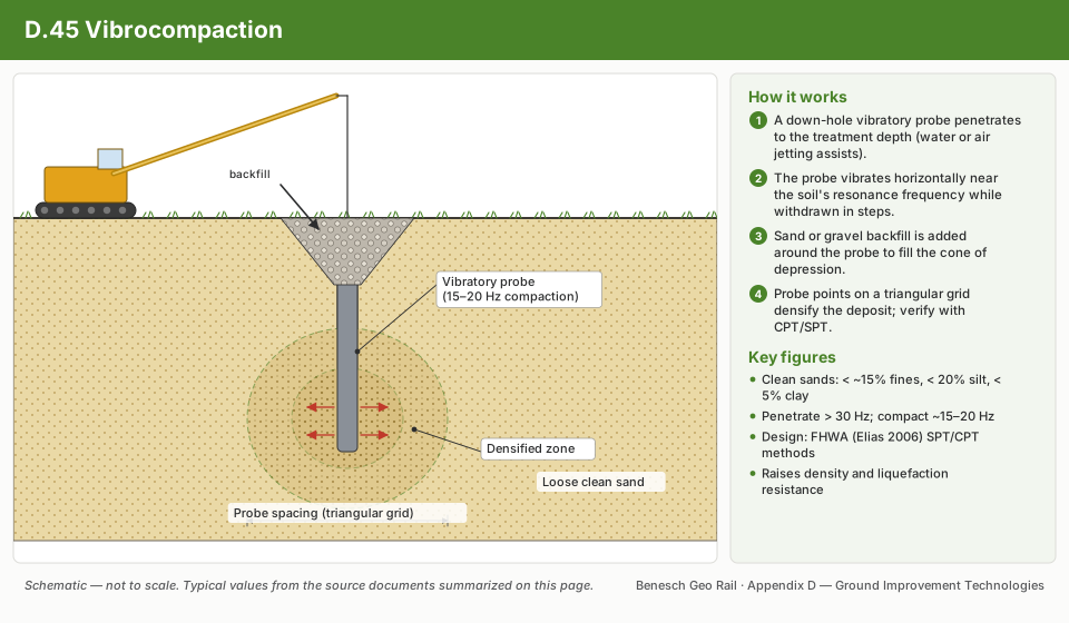
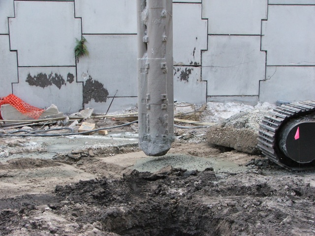
Vibrocompaction process
Withdrawal of vibratory probe
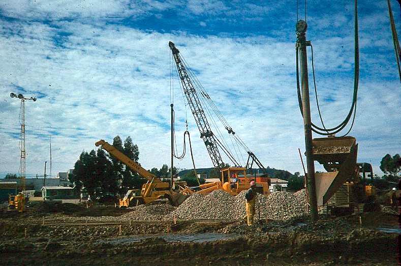
Sand compaction pile construction, Hollister CA
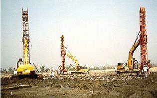
Blast densification — casing placement
17.2.3 Dynamic Compaction

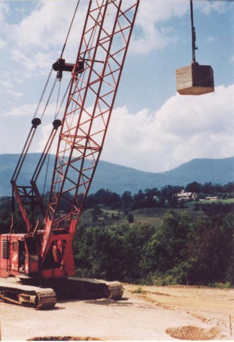
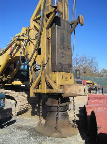
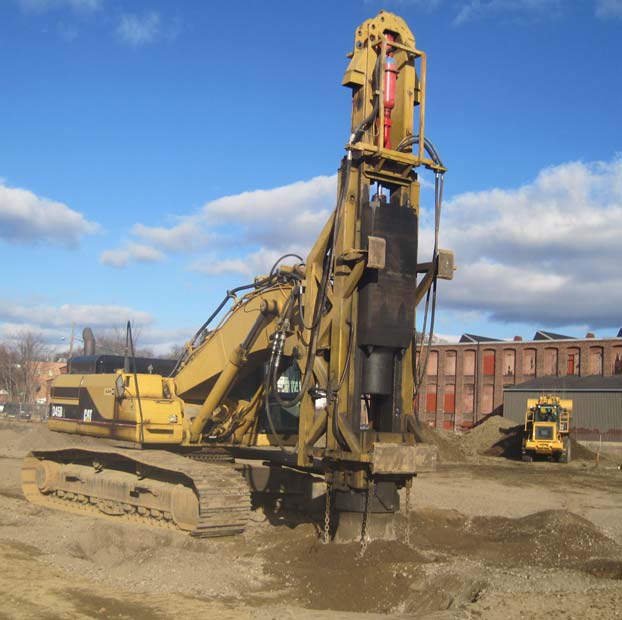
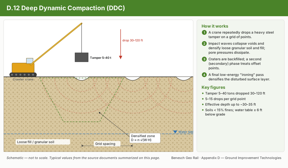
Dynamic compaction densifies loose fills and granular soils by repeated high-energy drops of a heavy pounder (10,000–30,000 lb) from heights of 30–90 ft.

Influence depth (Menard & Broise 1975):

D = n √Wh ⋅ H    (ft)

Where:

  • W_h = weight of pounder (tons)
  • H = drop height (ft)
  • n = empirical efficiency factor (0.35–0.65; 0.50 typical for saturated granular soil)

Energy per unit area:

E = ndrops ⋅ Wh ⋅ HAgrid    (ton·ft/ft²)

For railroad applications, dynamic compaction is restricted to areas beyond client setback from active track (Table 17-1). Vibration monitoring (Chapter 15) with a peak particle velocity (PPV) threshold of 0.5 in./s at the nearest track is required by UPRR and BNSF.

Reference graphics

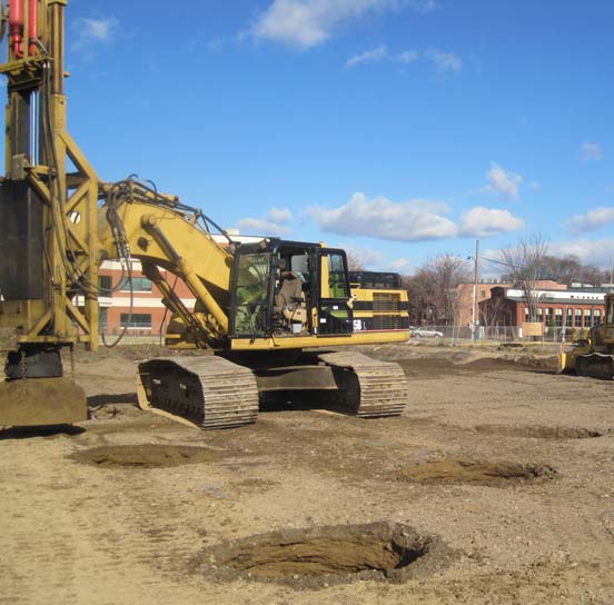
Dynamic compaction — crane and tamper
Dynamic compaction crater inspection
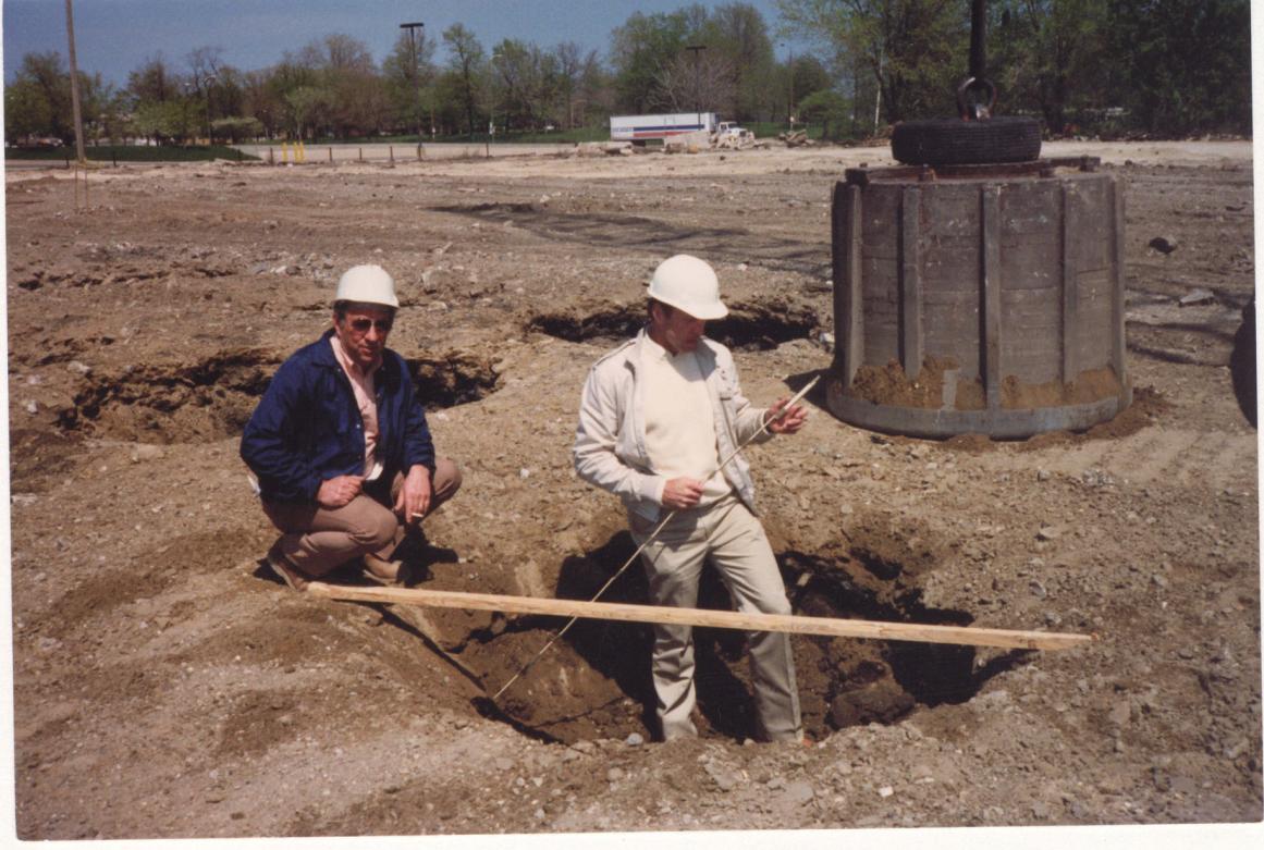
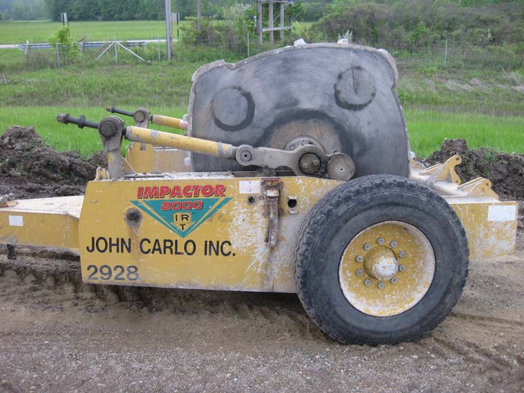
High-energy impact roller
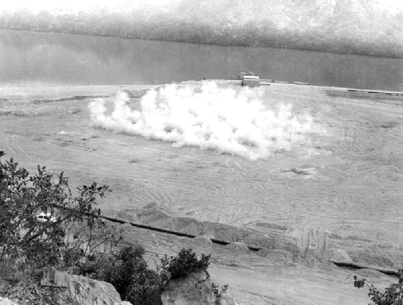
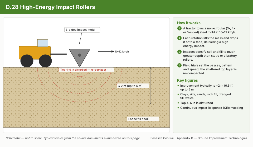
Blast densification — surface expression

Reference graphics · click to zoom

Dynamic Compaction
Dynamic Compaction
Rapid Impact Compaction — First Pass
Rapid Impact Compaction — Hammer and Anvil Foot
Rapid Impact Compaction in Progress
Supplemental reference · LEVI Library

What densification can realistically achieve

Table 17-S2. Upper-bound test values after deep dynamic compaction (GEC 13, Table 4-2, from FHWA 1986)

Soil typeSPT N (blows/ft)CPT qc (tsf)PMT limit pressure (tsf)
Pervious coarse-grained: sands and gravel30–50200–30020–25
Semipervious: sandy silts25–35135–17714.6–20
Semipervious: silts and clayey silts20–35104–13510.4–14.6
Partially saturated impervious: clay fill, mine spoil20–40*N/A14.6–20
Landfills15–40*N/A5.2–10.4

* Higher values may reflect large particles. These are maxima for estimating what is possible; verify actual improvement by testing while the equipment is still on site, and allow for delayed improvement as pore pressures dissipate.

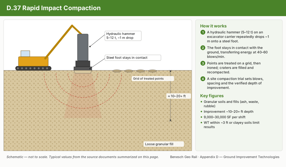
Rapid impact compaction (RIC) is a smaller-footprint alternative where the setbacks in Table 17-1 rule out a crane and pounder. A 5–9 ton weight on an excavator drops about 4 ft onto a 5-ft-diameter tamper at 40–60 blows/min. It densifies granular fills, ash and building waste to about 10–20+ ft and covers about 9,000–30,000 ft2 per shift. Groundwater should be at least 3 ft below the surface. It is not recommended for weak, low-permeability, clayey or high-fines soils. Energy and set per blow are recorded for QC, with SPT or CPT before and after for QA. Recorded peak noise was about 88 dBA. The depth of compaction cannot be controlled precisely.

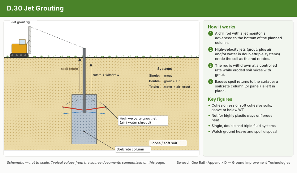
Jet grouting diameters reported by SHRP2 range from about 3 to 15 ft (larger than the 1.5–5 ft in Section 17.6.3, which reflects smaller systems). Depths are generally under 100 ft but exceed 160 ft in some cases. Soilcrete strength reflects the soil (higher in sands and gravels). Highly plastic clays and fibrous peat erode poorly and are not recommended. Spoil must be removed continuously, and surface or lateral movement must be watched — an important check beneath or next to track.

Source: Schaefer, V. R. et al. (2017). Ground Modification Methods Reference Manual, Vol. I. Geotechnical Engineering Circular No. 13, FHWA-NHI-16-027 · SHRP2 R02 / GeoTechTools (2012). Rapid Impact Compaction and Jet Grouting fact sheets

Technology sheets for this method · see 17.16 Technology Library

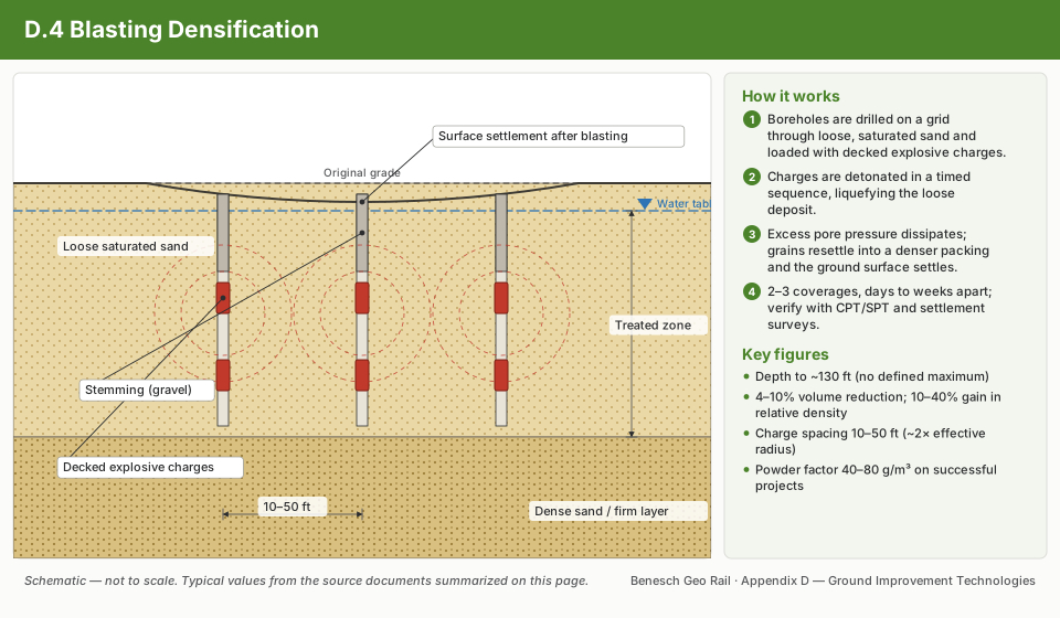
Traditional Compaction schematic17.16.42Traditional CompactionDeep Dynamic Compaction schematic17.16.12Deep Dynamic CompactionRapid Impact Compaction schematic17.16.37Rapid Impact CompactionHigh-Energy Impact Rollers schematic17.16.28High-Energy Impact RollersIntelligent Compaction schematic17.16.29Intelligent CompactionVibrocompaction schematic17.16.45VibrocompactionBlasting Densification schematic17.16.4Blasting Densification

Case study: 17.17.1 Measuring roller force with pile-driving monitors (Look 2023), in §17.17 Case Studies.

17.3 Prefabricated Vertical Drains (PVDs) with Staged Loading
17.3.1 Radial Consolidation Theory (Barron 1948)

PVDs accelerate consolidation by reducing the drainage path from the full layer thickness H_dr (vertical flow) to the horizontal spacing s_r between drains (radial flow). The average degree of consolidation from radial drainage U_r is:

Ur = 1 - exp[-8 Trμ]

Where T_r is the radial time factor:

Tr = ch ⋅ tde2

And:

  • c_h = horizontal coefficient of consolidation (ft²/day); typically 2–5× c_v for laminated clays
  • t = elapsed time (days)
  • d_e = equivalent diameter of influence zone (ft) = 1.13 × s for square grid; 1.05 × s for triangular grid; s = drain spacing (ft)
  • μ = drain spacing/smear/resistance factor:
μ = ln(dedw) - 34 + ds2de2 - ds2(khks - 1)ln(dsdw) + π kh ⋅ z(2L - z)qw

Where:

  • d_w = equivalent drain diameter (ft); standard PVD: d_w = 2(a + b)/π where a = 2 in., b = 4 in. → d_w = 0.196 ft
  • d_s = smear zone diameter (ft) = 2–3 × d_mandrel (typically 0.5 ft for standard mandrel)
  • k_h/k_s = horizontal to smear zone permeability ratio (typically 3–5)
  • q_w = drain discharge capacity (ft³/day); typically 0.5–2.0 ft³/day for standard PVD
  • L = drain length (ft); z = depth (ft)

For preliminary design, the simplified Hansbo (1981) formula is commonly used (omitting well resistance and smear):

μ ≈ ln(dedw) - 0.75
17.3.2 Combined Radial and Vertical Consolidation

The total degree of consolidation U_total combines radial and vertical drainage:

1 - Utotal = (1 - Ur)(1 - Uv)

Where U_v is from the Terzaghi vertical consolidation equation (Chapter 12, Section 12.7).

17.3.3 Staged Loading for Embankment Construction

Where subgrade shear strength s_u is insufficient for the full embankment load, construction proceeds in stages with PVDs to gain strength before next stage:

Strength gain from consolidation (Ladd 1991 SHANSEP):

su,consolidated = S ⋅ σ'v,consolidated ⋅ OCRm

Where S = 0.22–0.25 (normalized undrained strength ratio for soft clay); m = 0.88 (for CK₀U triaxial compression). For each stage: place fill to height H_i; wait for U_r ≥ 80% before next stage; verify FS_slope ≥ 1.3 (EOC) before next placement.

Table 17-2: PVD Design Parameters — Representative Railroad Embankment Cases
ProjectRailroadSoft Layer (ft)c_h (ft²/day)c_v (ft²/day)Drain Spacing (ft)GridTarget UtotalTime to Utarget
Coastal Georgia MainlineCSXT350.0120.0065.0Triangle90%120 days
Manitoba Prairie FillCPKC280.0180.0094.5Square85%90 days
Louisiana Yard ExpansionBNSF420.0150.0085.0Triangle90%150 days
Quebec Mainline Soft ClayCN500.0100.0054.0Triangle90%180 days
NEC Embankment WideningAmtrak200.0220.0114.0Square95%75 days

Wick drains in rail work

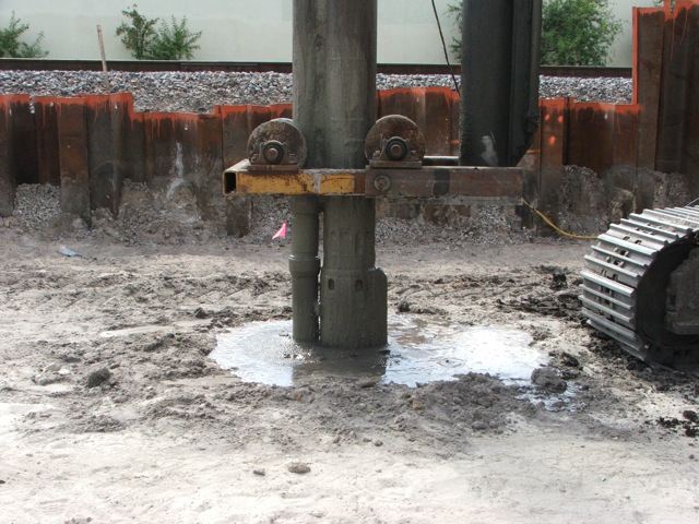
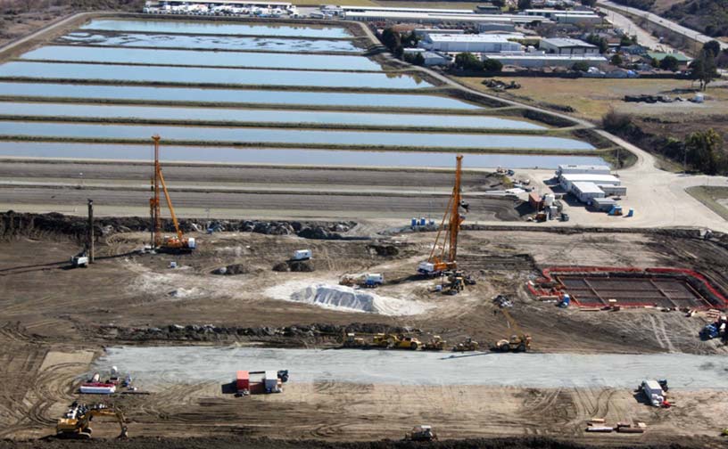
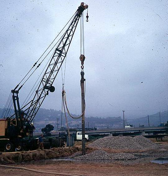
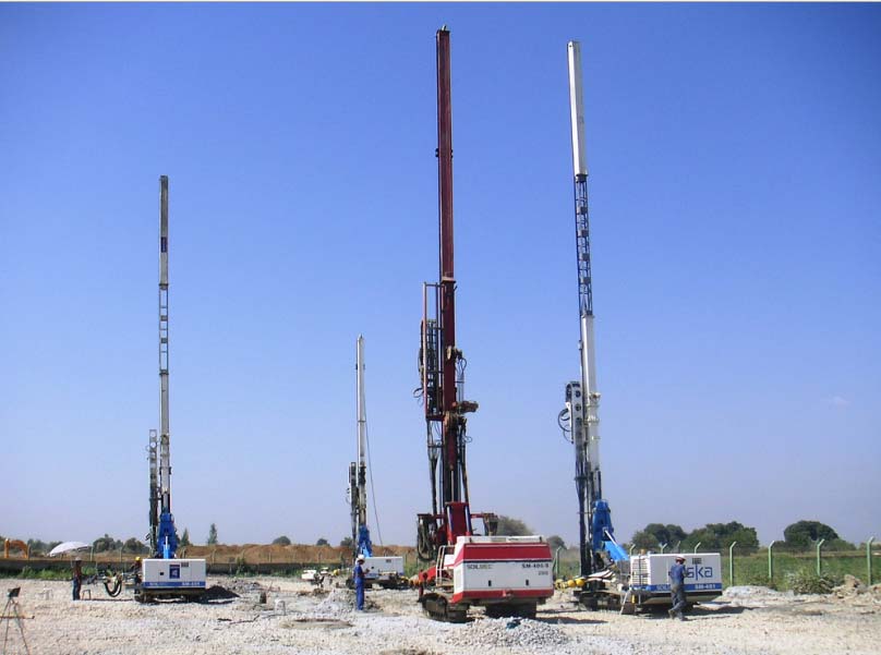
Wick drains give trapped pore water a short vertical path out, accelerating consolidation of soft saturated ground that would otherwise take years to drain. Several mandrels can work a large site at once.

Figures · click to zoom

Figure 17-14. Wick-drain installation rigs.

After Geotechnology for Railroaders Program, Module 6.2; §02. Full reference under Supplemental Sources.

Technology sheets for this method · see 17.16 Technology Library

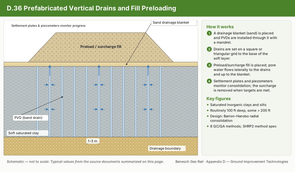
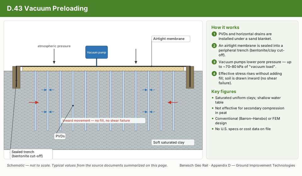
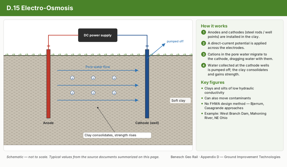
Prefabricated Vertical Drains and Fill Preloading schematic17.16.36Prefabricated Vertical Drains and Fill PreloadingVacuum Preloading with and without Prefabricated Vertical Drains schematic17.16.43Vacuum Preloading with and without Prefabricated Vertical DrainsElectro-Osmosis schematic17.16.15Electro-Osmosis

Case study: 17.17.2 Wick-drain rigs on dredged sand over 104 psf clay: four ways to size the platform (Look 2023), in §17.17 Case Studies.

17.4 Stone Columns
17.4.1 Priebe Method for Composite Modulus

Stone columns (vibro-replacement) improve soft cohesive subgrades by inserting dense granular columns (typically 24–36 in. diameter) on a regular grid. The Priebe (1995) method computes an improvement factor n₀ based on area replacement ratio A_c/A:

Area replacement ratio:

as = AcA = π Dc2 / 4scol2    (square grid)

Where D_c = column diameter (ft); s_col = column spacing (ft).

Basic improvement factor (Priebe 1995):

n0 = 1 + as [1as Ka ⋅ (1 - as)(1 - 2νs)1 - νs - 1]-1

Simplified for ν_s = 0.33 (stone column internal friction coefficient assumed φ'_col = 40°, K_a = tan²(45 − 20) = 0.217):

n0 ≈ 1 + as [12 as + (1 - as)/2 - 1]    (approximation)

Composite settlement reduction:

SimprovedSuntreated = 1n0

Composite modulus:

Ecomposite = EsoilSimproved/Suntreated = n0 ⋅ Esoil

Reference graphics

Stone column construction with vibro rigs
Crane-suspended vibroflot and stone backfill
Geotextile-encased sand column installation
Vibro concrete column installation
17.4.2 Load-Carrying Capacity of Stone Column Group

The bearing capacity of the composite improved ground beneath a loaded area is:

qult,composite = as ⋅ qult,col + (1 - as) ⋅ qult,soil

Where q_ult,col = bearing capacity of stone column material (typically 8–15 tsf); q_ult,soil = undrained bearing capacity of surrounding clay (N_c × s_u; typically 1–3 tsf).

Table 17-3: Stone Column Design Parameters — Railroad Applications
ApplicationD_c (in.)Spacing (ft)a_sn₀ (Priebe)Settlement Reductionφ'_col (°)
Track subgrade support247.50.0571.6–1.844–56%38–42
Intermodal yard (light)308.00.0771.8–2.245–55%40
Bridge abutment366.00.1962.5–3.560–71%40–42
Crane runway (RTG)365.00.2833.0–4.067–75%42
Surcharge preload zone249.00.0401.4–1.638–44%38

Reference graphics

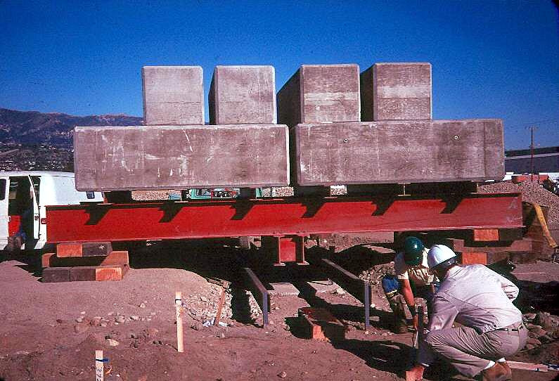
Kentledge load test on improved ground
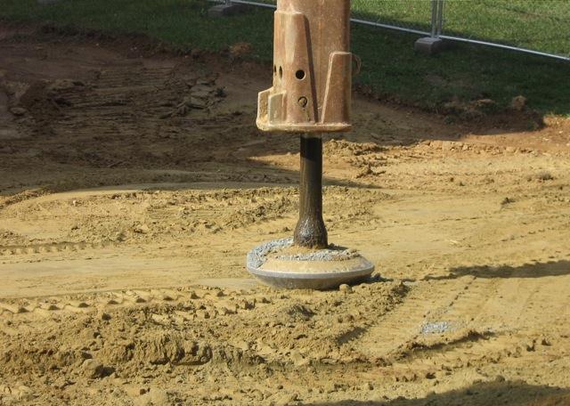
Rammed aggregate pier tamper foot
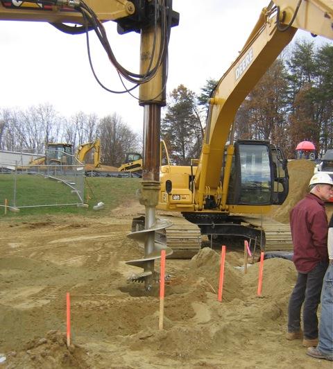
Aggregate pier drilling with auger

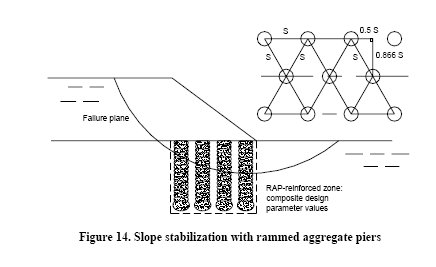
Rammed aggregate piers through a slip surface

Stone columns and rammed aggregate piers installed on a triangular grid through a shallow-to-medium failure plane create a composite of native soil and dense columns that carries load and resists shear better than either alone.

Figures · click to zoom

Figure 17-15. Slope stabilization with rammed aggregate piers on a triangular grid.

After Geotechnology for Railroaders Program, Module 6.1; §07. Full reference under Supplemental Sources.

Technology sheets for this method · see 17.16 Technology Library

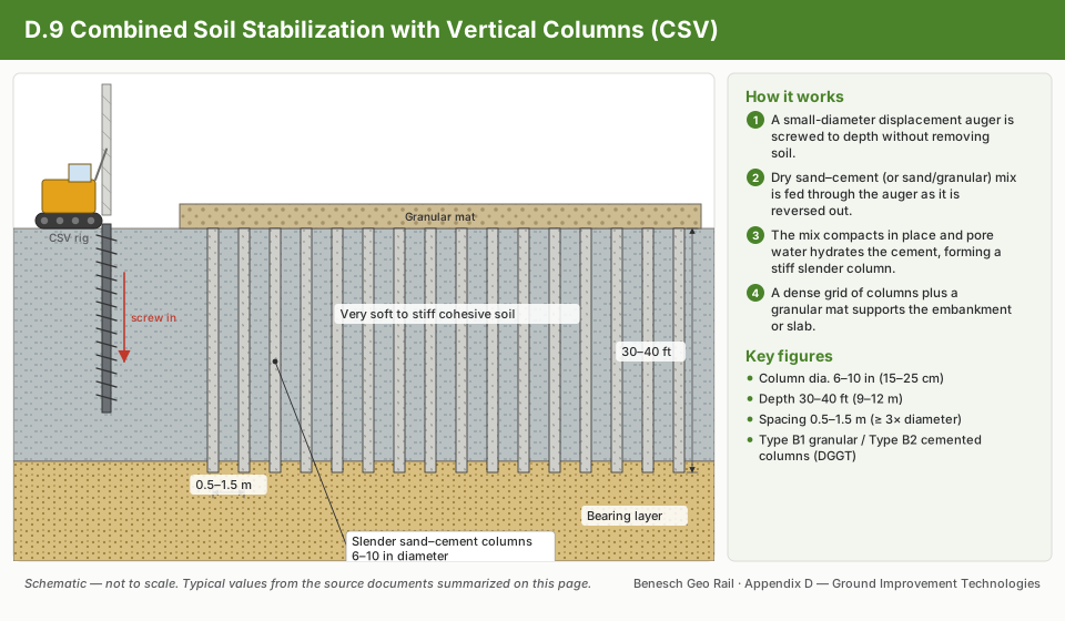
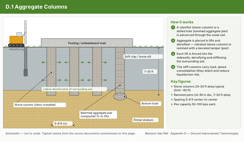
Aggregate Columns schematic17.16.1Aggregate ColumnsGeotextile Encased Columns schematic17.16.26Geotextile Encased ColumnsSand Compaction Piles schematic17.16.38Sand Compaction PilesVibro-Concrete Columns schematic17.16.44Vibro-Concrete ColumnsCombined Soil Stabilization with Vertical Columns schematic17.16.9Combined Soil Stabilization with Vertical ColumnsColumn-Supported Embankments schematic17.16.8Column-Supported Embankments
17.5 Deep Soil Mixing (DSM)
17.5.1 Method Description

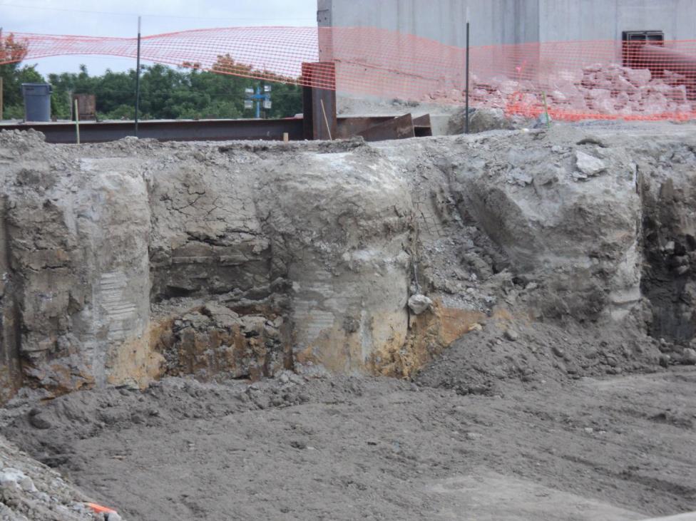
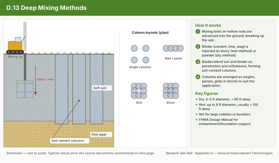
DSM mechanically blends in-situ soil with cementitious binder (Portland cement, lime, or blends) using hollow-stem augers with injection ports. The resulting soil-cement mass (referred to as a "treated mass" or "column") achieves unconfined compressive strengths of 50–300 psi depending on binder content and soil type. DSM is used for:

  • Soft clay improvement beneath railroad embankments (treated mass beneath track)
  • Liquefaction mitigation (Chapter 14, Worked Example 9-1)
  • Lateral support walls for excavations adjacent to track
  • Embankment toe walls to prevent lateral spreading

Design unconfined compressive strength:

qu = flab × qu,field

Where f_lab = 0.20–0.33 (field-to-laboratory strength ratio; use 0.25 for conservative preliminary design). Laboratory mix design targets q_u,lab ≥ 100 psi for soft clay treatment.

Reference graphics

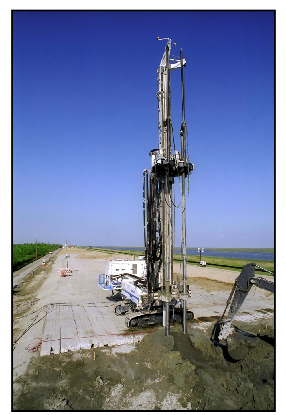
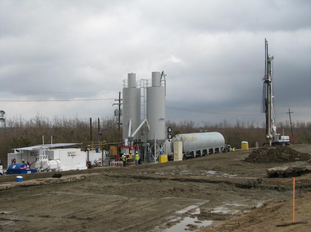
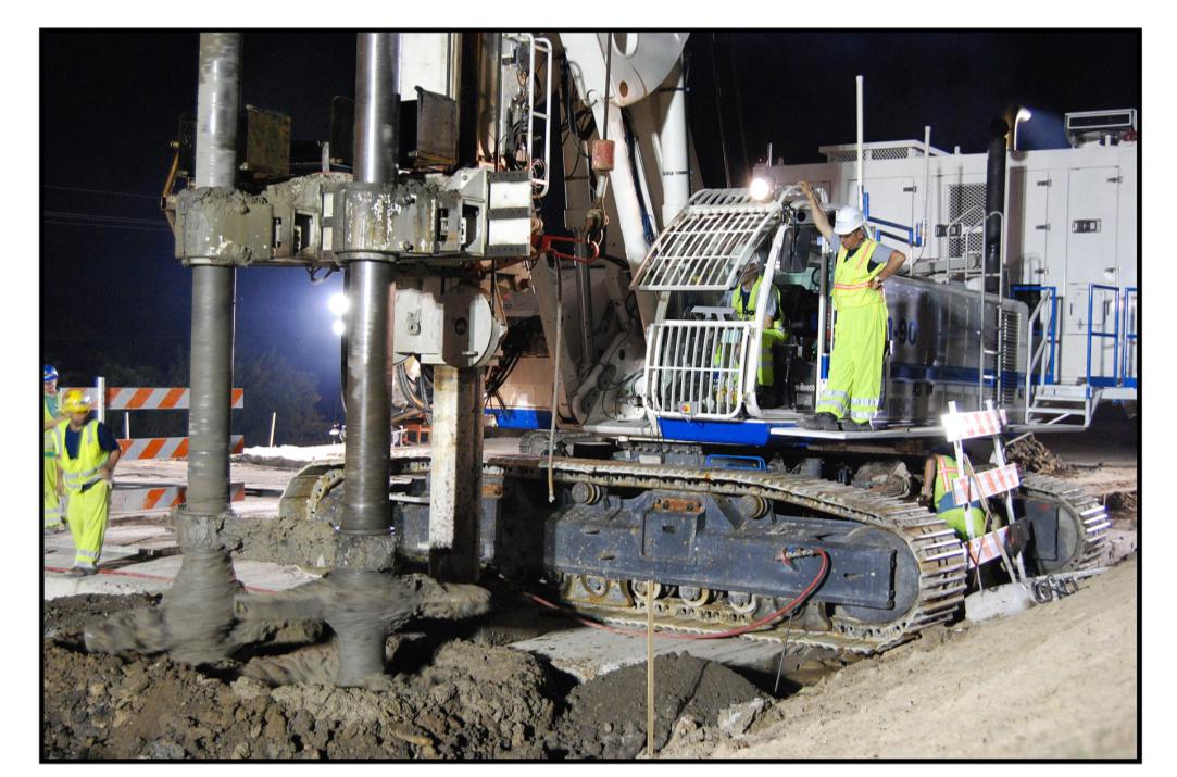
Deep mixing rig on levee, New Orleans
DSM batch plant and mixing rig
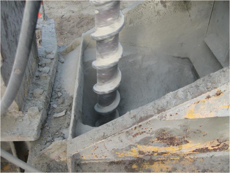
Close-up of deep soil mixing tool
Cement-soil column auger and cement hopper
17.5.2 Composite Modulus for DSM Treatment

Treated mass elastic modulus:

EDSM = 150 ⋅ qu,field    to    500 ⋅ qu,field    (psi)

Typical range: E_DSM = 3,000–30,000 psi. For settlement reduction using composite modulus approach:

Ecomposite = aDSM ⋅ EDSM + (1 - aDSM) ⋅ Esoil

Where a_DSM = area replacement ratio of DSM columns within the treated zone (typically 0.15–0.35 for track subgrade improvement).

Reference graphics

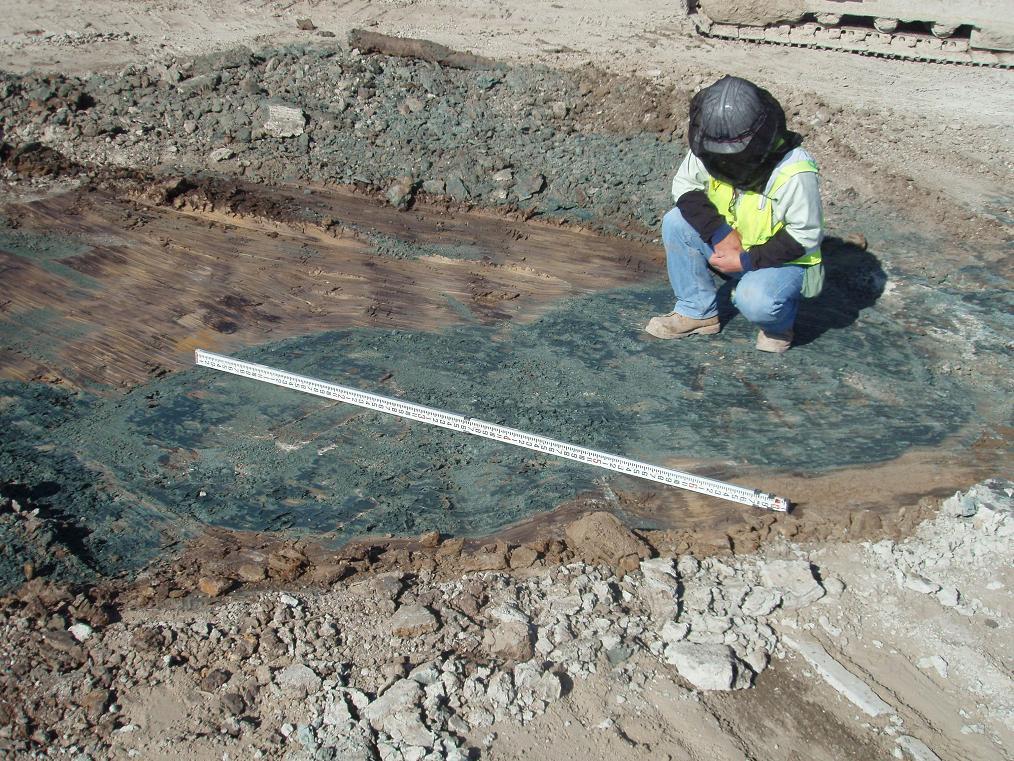
Exposed tops of DSM columns
Exposed sides of DSM columns
17.5.3 Minimum Strength Criteria by Client
Railroadq_u,field minimum (psi)Test MethodCuring Period (days)Notes
UPRR50ASTM D216628Liquefaction mitigation: 75 psi
BNSF50ASTM D216628Track subgrade: 28-day cure
Amtrak75ASTM D216628NEC: higher strength for vibration control
CN60ASTM D216628Bridge abutment zone: 90 psi
CPKC60ASTM D216628Freeze-thaw durability check required
CSXT50ASTM D216628Southeast soft clays
NSR50ASTM D216628Appalachian foothill colluvium
G&W45ASTM D216628Short-line: minimum acceptable
AREMA50ASTM D216628MRE Ch. 1 baseline
Supplemental reference · LEVI Library

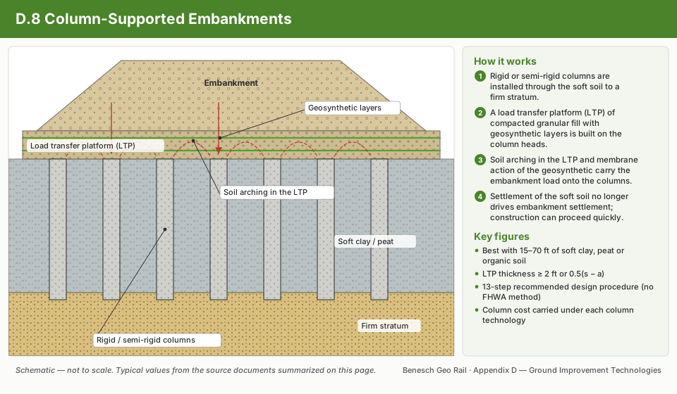
Column-supported embankments (CSE) and load transfer platforms

When there is no time to preload, columns of almost any type — aggregate piers, vibro-concrete columns, DSM columns, augered or driven piles — can carry the embankment to a firm layer. SHRP2 R02 notes that the method is most economical for 15–70 ft of soft clay, peat or organic soil, and cites the Rancocas Creek Railroad Bridge approach in New Jersey (Figure 17-S3). Key points of the recommended design procedure (there is no approved FHWA method):

  • Design the columns to carry the entire embankment plus surcharge (commonly 250–300 psf). SHRP2 recommends an allowable post-construction settlement of 3 in.; track tolerances in Chapter 12 may govern tighter.
  • The embankment must exceed a critical height (below which differential settlement shows at the surface), and clear span s − a ≤ 10 ft (a = pile-cap width, or 0.886 dcol for round columns).
  • A geosynthetic-reinforced load transfer platform is typical where spacing exceeds about 5 ft. Thickness should be at least 2 ft and at least 0.5(s − a). Use select fill with φ′ ≥ 35°, graded 100% passing 4 in., 15–70% passing No. 4, 10–60% passing No. 40 and 5–15% passing No. 200, with LL < 40 and PI < 20. Place at least two reinforcement layers with 3-ft overlaps.
  • Check global stability (FS ≥ 1.5 recommended with LTPs) and lateral spreading of the reinforcement. Closely spaced aggregate columns often need no LTP.

Table 17-S3. Typical allowable column capacities (SHRP2, adapted from Elias et al., 2006)

Column typeAllowable capacity (kip)Typical length (ft)Diameter/width (in.)
Stone columns20–11010–3518–47
Geotextile-encased columns65–13510–3530–60
Rammed aggregate piers50–15010–3524–36
Augered piles75–25015–8012–24
Vibro-concrete columns100–25010–3518–24
Deep mixing columns90–27030–10024–120
Precast concrete piles90–22530–50up to 24
Steel H / pipe piles90–450 / 180–55015–100 / 30–1306–12 / 8–48

Source: SHRP2 R02 / GeoTechTools (2012). Column-Supported Embankments — fact sheet, design guidance and photographs

Supplemental figures · LEVI Library
Completed T-Wall column-supported embankment for the Rancocas Creek railroad bridge approach, New Jersey (SHRP2 GeoTechTools).
Supplemental Figure 17-S3. Completed T-Wall column-supported embankment for the Rancocas Creek railroad bridge approach, New Jersey (SHRP2 GeoTechTools). Source: SHRP2 R02 / GeoTechTools (2012). Column-Supported Embankments — fact sheet, design guidance and photographs.
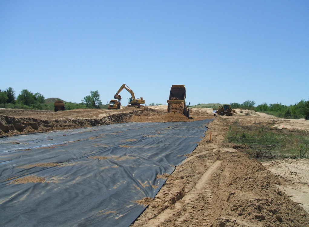
Placement of geosynthetic reinforcement for a load transfer platform over columns (SHRP2 GeoTechTools).
Supplemental Figure 17-S4. Placement of geosynthetic reinforcement for a load transfer platform over columns (SHRP2 GeoTechTools). Source: SHRP2 R02 / GeoTechTools (2012). Column-Supported Embankments — fact sheet, design guidance and photographs.

Technology sheets for this method · see 17.16 Technology Library

Deep Mixing Methods schematic17.16.13Deep Mixing MethodsCombined Soil Stabilization with Vertical Columns schematic17.16.9Combined Soil Stabilization with Vertical ColumnsColumn-Supported Embankments schematic17.16.8Column-Supported Embankments
17.6 Grouting Methods
17.6.1 Compaction Grouting

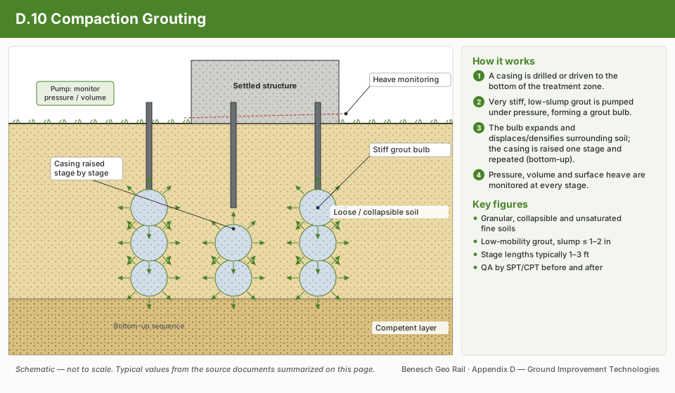
Compaction grouting injects a stiff grout (slump < 2 in.) that does not penetrate soil pores but instead forms a grout bulb, displacing and densifying surrounding soils. Used for:

  • Densification of loose fills beneath existing track (UPRR, BNSF historical mainline settlement)
  • Foundation underpinning adjacent to active track
  • Correction of localized subgrade settlement

Grout volume per bulb:

Vgrout = π6 Dbulb3    (ft3)

Where D_bulb = target bulb diameter (ft); typically 1.5–2.5 ft. Injection spacing = 4–8 ft on grid; primary and secondary passes used to achieve uniform densification.

Reference graphics

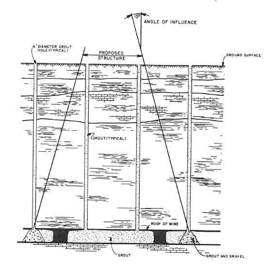
Grouting of abandoned mine voids beneath a structure
17.6.2 Permeation Grouting

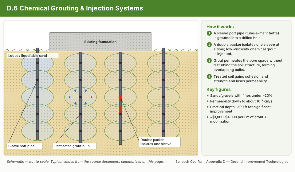
Low-viscosity grout (sodium silicate, acrylamide, or ultrafine cement) is injected under low pressure to penetrate pore spaces without disturbing soil fabric. Used in granular soils (D₁₅ > 0.025 in.) to reduce permeability or improve strength.

Groutability ratio (GR):

GR = D15,soilD85,grout ≥ 24    (for successful permeation)

Reference graphics

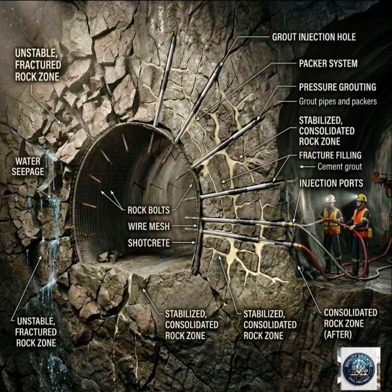
Pressure grouting of fractured rock
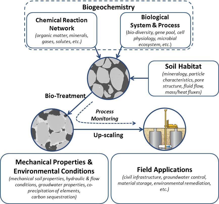
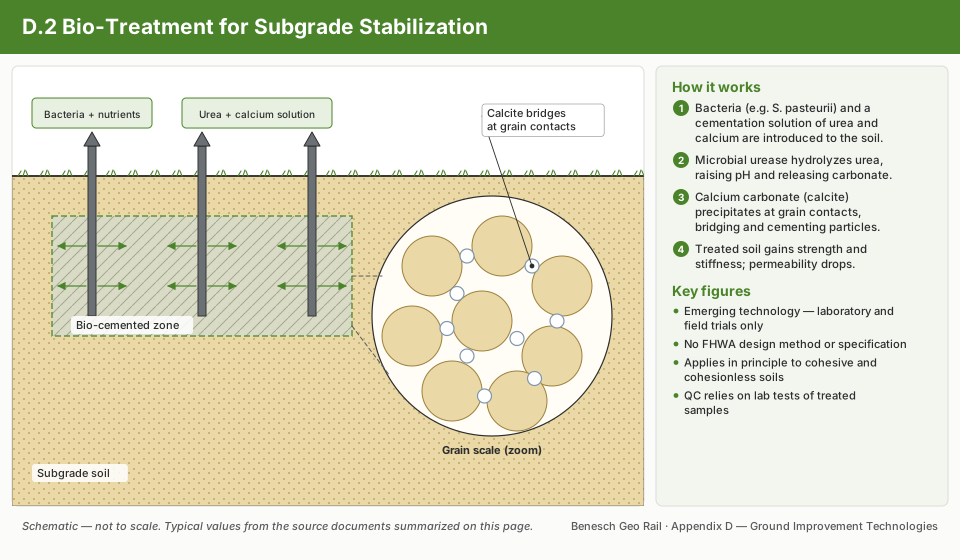
Bio-mediated soil treatment overview
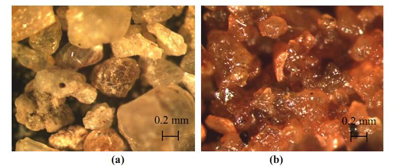
Untreated vs bio-cemented sand (microscope)

Groutability limits for permeation grouting

  • Cement and clay grouts suit sands and gravels only. They do not suit silts or clays, or soils with more than about 10% fines.
  • Silicate chemical grouts reach coarse silts and medium to fine sands.
  • Check the particle-size ratio: D15(soil) ≥ 25 × D85(grout).

After Selig & Waters (1994), ch. 11. Full reference under Supplemental Sources.

17.6.3 Jet Grouting

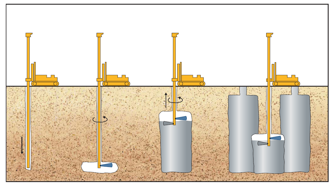
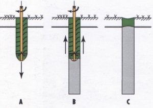
High-pressure jetting (3,000–7,000 psi) simultaneously erodes and mixes in-situ soil with cement grout, creating cylindrical treated columns. Single-fluid, double-fluid, and triple-fluid systems produce column diameters of 1.5–5.0 ft. Used by Amtrak for underpinning NEC structures and by UPRR/BNSF for liquefaction mitigation under existing embankments.

Column diameter (approximate, triple-fluid system):

Dcol ≈ 0.3 + 0.9 ⋅ Pjet0.5    (ft, for P in ksi)

Reference graphics

Jet grouting process

Reference graphics · click to zoom

Jet Grouting — Multiple Rigs Operating
Supplemental reference · LEVI Library

Slurry pressure injection under live track

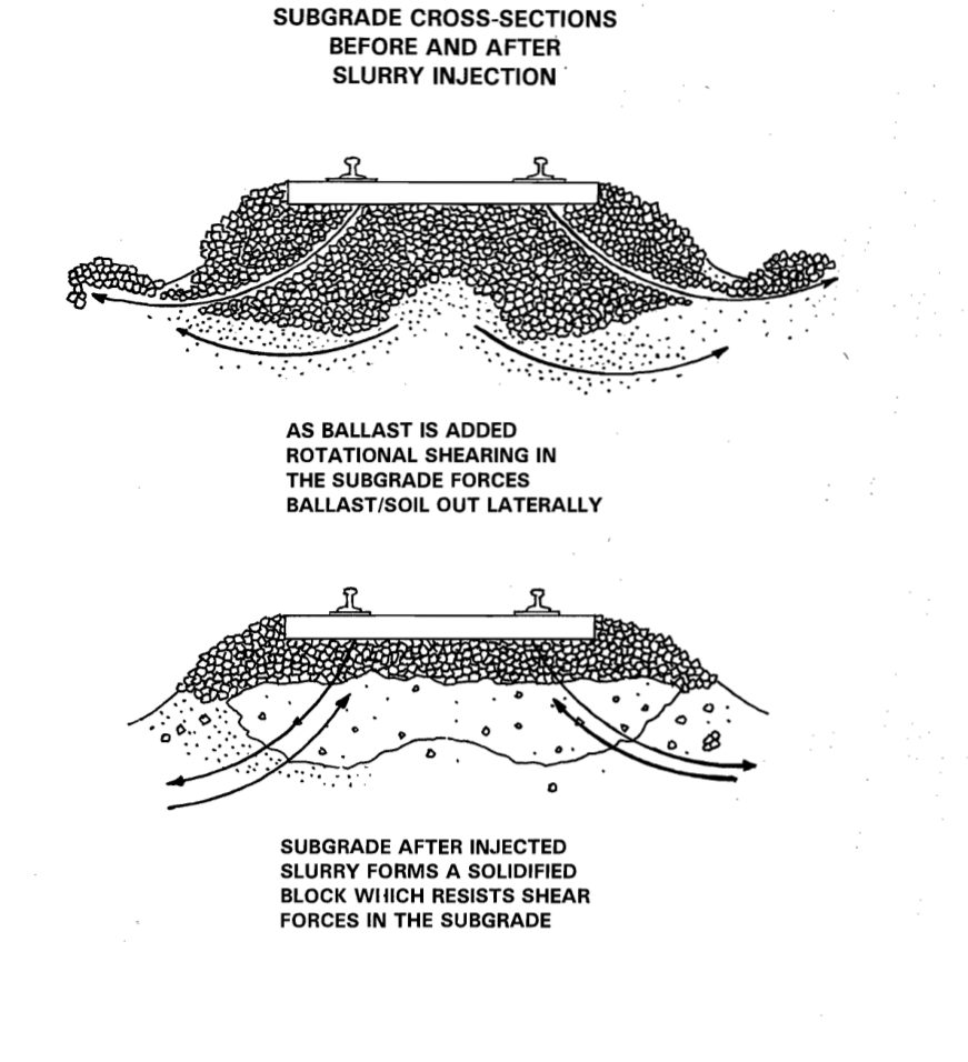
The grouting methods above are general. The method developed specifically for railroad subgrades is slurry pressure injection from hi-rail equipment, which can clear for trains between injections. Soft fine-grained subgrade and repeated resurfacing drive ballast down into ballast pockets that trap water, cause squeezes and keep the soil weak. Injection works in two ways:

  • Mechanical (void filling): a slurry heavier than water displaces trapped water from the pockets and sets into a ballast–grout block that resists the progressive shear (Figure 17-S1). Railroad cements (about 70–80% finely ground limestone, 20–30% cement clinker) reach up to about 1,000 psi; lime/fly ash up to about 125 psi. Slurry specific gravity should be at least 1.25.
  • Chemical (lime): hydrated or quicklime slurry travels along fissures, slickensides and shear planes and reacts with the clay. Lime slurry does not set on its own. Results may take 6–9 months to appear as lime migrates into the soil. Pengelly reports a CPT-measured average shear strength increase of 308% ten months after lime/fly ash injection.

Table 17-S1. Typical injection parameters (FRA handbook, 1977, and Pengelly)

ParameterTypical value
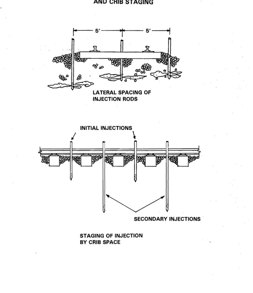
RodsThree, 5 ft apart: one on track centerline, one each side (Figure 17-S2)
DepthLime: 10–16 ft historically; most programs ≥ 20 ft; modern units 30–40 ft
Longitudinal spacingAbout 5 ft (every second or third crib; never more than 4 crib spaces); every crib, staged, in severe distress
Stage interval18–24 in., injecting downstage (top down) to refusal or target take
Pump pressure50–250 psi (150 psi common); keep low to maximize take
Lime slurry2.5–3 lb lime per gallon of water (never > 4); SG about 1.15–1.17
Quantity30–50 gal per track ft for a 10–16 ft lime injection (FRA); 200–250 lb dry solids per track ft typical, 150 mild to 1,000 severe (Pengelly)
StagingSecond or third pass 48 hr or more later into skipped cribs, e.g., deep lime pass then shallow void-filling pass

Investigation and testing. The FRA handbook suggests about 2 + L/250 borings for L up to 1,000 ft of problem track, 6 + (L − 1,000)/300 for 1,000–4,000 ft, and 16 + (L − 4,000)/400 for 4,000–10,000 ft, with continuous Shelby tubes for 5 ft just below the ballast and borings at least 5 ft below the deepest planned injection. Lab “lime-inoculated” specimens (1% lime by dry weight, representing 5-ft centers) are compared with untreated controls in swell, consolidation and strength tests. CPT before and after injection locates ballast pockets, sets the target take and verifies improvement. Hayward Baker case histories (Des Moines–Sioux City, every other crib, 14–40 ft; St. Joseph, MO, every crib to 20 ft after CPT found weak soil to 18–20 ft) used this approach. The FRA handbook itself cautions that results cannot yet be predicted reliably from lab tests and recommends a field test section before a program.

Material caution: Pengelly attributes past poor results partly to substandard fly ash and recommends only ash that reliably sets (Class C in his experience). Test every ash source for compatibility. Note that his description of the coal sources is reversed relative to ASTM C618, where Class F comes from bituminous or anthracite coal and Class C from sub-bituminous or lignite.

Source: Blacklock, J. R. and Lawson, C. H. (1977). Handbook for Railroad Track Stabilization Using Lime Slurry Pressure Injection. FRA/ORD-77/30, Federal Railroad Administration · Pengelly, A. D. Injection for Railroad Subgrades. Hayward Baker, Inc. (scanned; text recovered by OCR) · Hayward Baker, Inc. Railroad Subgrade Stabilization (brochure)

Supplemental figures · LEVI Library
Subgrade cross-sections before and after slurry injection: ballast pockets forcing lateral shear (top) and the solidified ballast&ndash;slurry block resisting shear (bottom).
Supplemental Figure 17-S1. Subgrade cross-sections before and after slurry injection: ballast pockets forcing lateral shear (top) and the solidified ballast–slurry block resisting shear (bottom). Source: Pengelly, A. D. Injection for Railroad Subgrades. Hayward Baker, Inc. (scanned; text recovered by OCR).
Injection rod spacing across the track (5 ft) and crib staging of initial and secondary injections.
Supplemental Figure 17-S2. Injection rod spacing across the track (5 ft) and crib staging of initial and secondary injections. Source: Pengelly, A. D. Injection for Railroad Subgrades. Hayward Baker, Inc. (scanned; text recovered by OCR).

Injection and grouting from the track

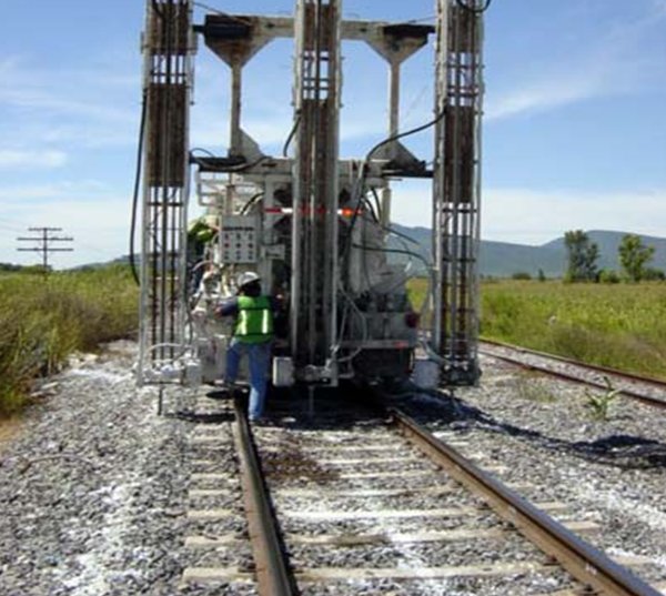
Cement-slurry injection and compaction grouting pump material into the ground under pressure, densifying loose soil or filling voids without excavating the track. Where poor material is shallow, remove-and-replace with engineered granular fill over a separator geotextile is still the most direct fix. Admixture stabilization, usually with Portland cement, treats soil in place, and is faster and cheaper when the soil responds well.

Figures · click to zoom

Figure 17-16. Rail-mounted cement-slurry injection rig.
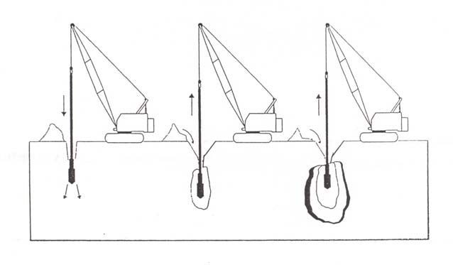
Figure 17-17. Compaction grouting and dynamic compaction concept.

After Geotechnology for Railroaders Program, Module 6.2; §04–05. Full reference under Supplemental Sources.

Technology sheets for this method · see 17.16 Technology Library

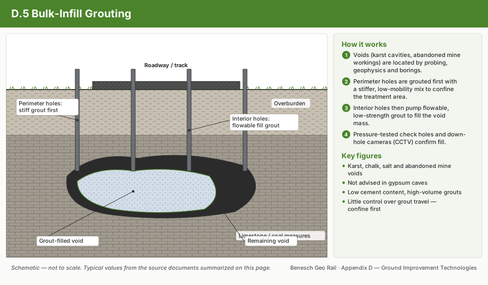
Compaction Grouting schematic17.16.10Compaction GroutingJet Grouting schematic17.16.30Jet GroutingChemical Grouting & Injection Systems schematic17.16.6Chemical Grouting & Injection SystemsBulk-Infill Grouting schematic17.16.5Bulk-Infill Grouting
17.7 Lime and Cement Stabilization
17.7.1 Lime Stabilization

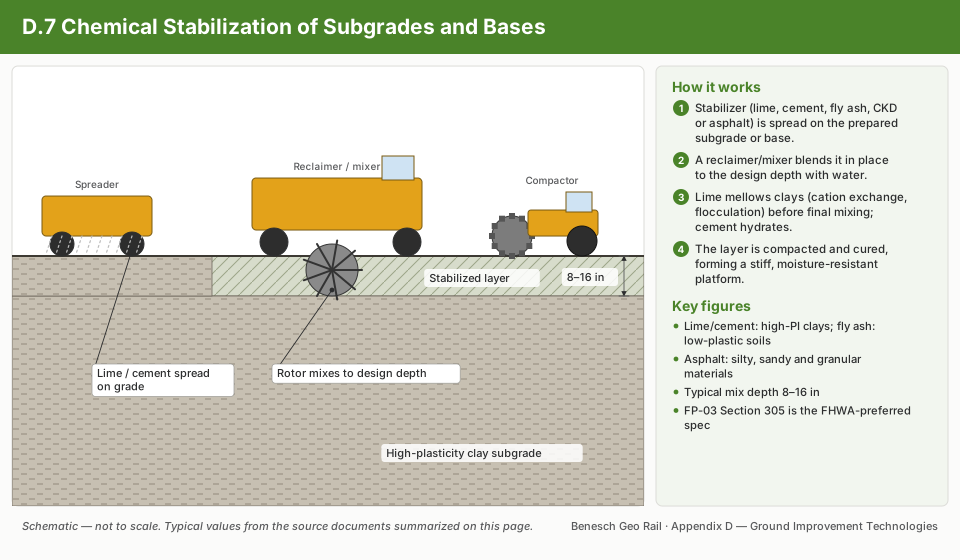
Hydrated lime (Ca(OH)₂) added to fine-grained soil produces immediate PI reduction through cation exchange and flocculation, and long-term pozzolanic strength gain.

PI reduction rule of thumb:

PIfinal ≈ PIinitial - 5 ⋅ Lp

Where L_p = lime percentage (by dry soil weight, %). Target: PI_final < 12 for use as subgrade; PI_final < 20 for use as embankment fill. Minimum lime content: 3%; maximum practical: 8%.

Strength gain timeline:

Curing Timeq_u (psi) — Typical CL/CH Clayq_u (psi) — ML/MH Silt
1 day15–3010–20
7 days30–8020–50
28 days50–15035–90
1 year100–30070–200

Sulfate precaution: For sulfate content SO₄ > 2,000 ppm (ASTM D4327), lime-treated clay may experience delayed ettringite formation causing swell of 3–10%. In such cases, use cement or fly-ash binder instead.

Reference graphics

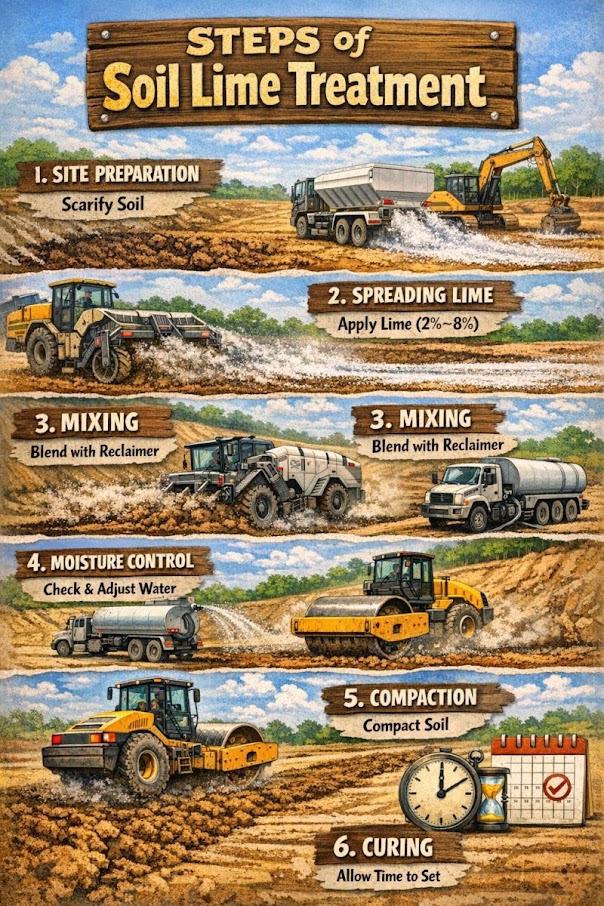
Steps of Soil Lime Treatment
17.7.2 Cement Stabilization

Portland cement (ASTM C150, Type I/II) or fly ash (ASTM C618, Class C or F) stabilizes both granular and fine-grained soils through cementation. Design target: q_u ≥ 200–300 psi at 7 days (ASTM D1633) for pavement base applications (Chapter 18).

Mix design proportioning:

qu = f[ccement, soil type, wc, tcure]

Determined from laboratory trial mixes at cement contents of 4%, 6%, 8%, 10% by dry weight. Minimum cement content for railroad fill: 4% (AREMA MRE Chapter 1 Specification).

Reference graphics

Cement Treated Base (CTB)
Supplemental reference · LEVI Library

Sulfate thresholds and construction steps (National Lime Association)

Correction to Section 17.7.1. The sulfate problem is not specific to lime. Sulfates react with calcium and clay alumina to form expansive ettringite and thaumasite with any calcium-based additive — lime, portland cement or fly ash. Switching to cement or fly ash therefore does not avoid it. NLA guidance:

Soluble sulfateGuidance
< 3,000 ppm (0.3%)Unlikely to cause problems
3,000–5,000 ppmReadily stabilized with good practice: plenty of water, ample mellowing between mixings
> 5,000 ppmOften two lime applications: first before mixing, second after a multi-day mellowing at about 5% over optimum moisture so that ettringite forms before compaction (research cited suggests a single application at +2% moisture up to 7,000 ppm)

Sulfates occur in isolated seams and pockets (commonly naturally occurring gypsum in the western U.S., or industrial and synthetic-gypsum contamination), so sample more densely than for other index tests. Other NLA criteria: good candidates have at least 25% passing No. 200 and PI > 10; organics > about 1% need extra lime or special procedures; subgrade stabilization typically uses 3–6% lime. Construction sequence: scarify and pulverize, spread lime, preliminary mix and water, mellow 1–7 days, final mix until 100% of non-stone material passes 1 in. and at least 60% passes No. 4, compact, then moist- or membrane-cure. For embankment repairs, treat borrow in a stockpile at 1–3% over optimum so mellowing happens off the critical path.

Source: National Lime Association (2004). Lime-Treated Soil Construction Manual: Lime Stabilization & Lime Modification, Bulletin 326

Stabilized subgrade under track in frost areas

In seasonal-frost areas, use lime or cement stabilized subgrade under track with caution. Use it only after a laboratory program on the treated soil that includes a frost-susceptibility test and a freeze–thaw durability test. UFC 4-860-01FA refers to TM 5-822-14 for the design and construction of soil-stabilized subgrades.

After UFC 4-860-01FA (2004), ch. 6, §8e. Full reference under Supplemental Sources.

Choosing cement, lime or bitumen for trackbed soils

Table 17-SW1. Admixture screening criteria
AdmixtureSuitable soilsAvoid / notes
CementBroadly graded sand–gravel; < 35% passing No. 200 and PI < ~30Highly organic, high-salt or high-sulfate soils; coarse gravel (high cement demand); CH clay (hard to mix). Use lime instead where the fines or PI limits are exceeded.
LimeClay fraction (< 2 µm) ≥ 7% and PI > 10; typically 3–7% lime by weightLab reactivity test required. Lowers maximum dry density and raises optimum moisture, which helps wet clay. Strength gains slowly, giving a flexible working time, but it is not for a rapid strength need.
BitumenGW, GP, SW, SP, GM, SMPoor in wet soils. Too much bitumen lowers strength. A sprayed emulsion film works only where the water table will not be trapped beneath it.

Cracking risk. A cement-stabilized layer over softer soil develops tension at its base under each axle. Unlike a granular layer, it cannot build up residual compression, so it may crack and lose its benefit. Lime-treated soil cracks less than soil-cement. Cement also raises wet–dry and freeze–thaw resistance and lowers swell. It reduces permeability in granular soils but can increase it in clay.

After Selig & Waters (1994), ch. 11. Full reference under Supplemental Sources.

Technology sheets for this method · see 17.16 Technology Library

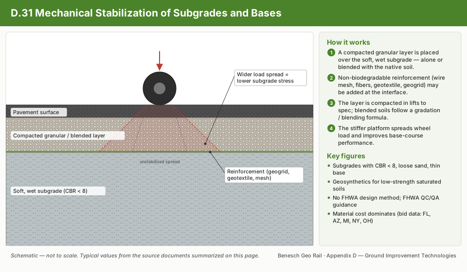
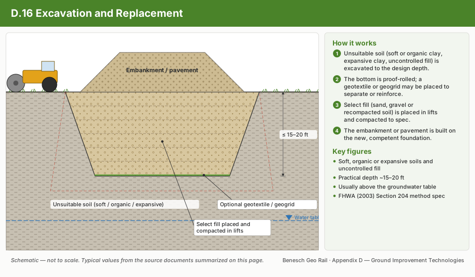
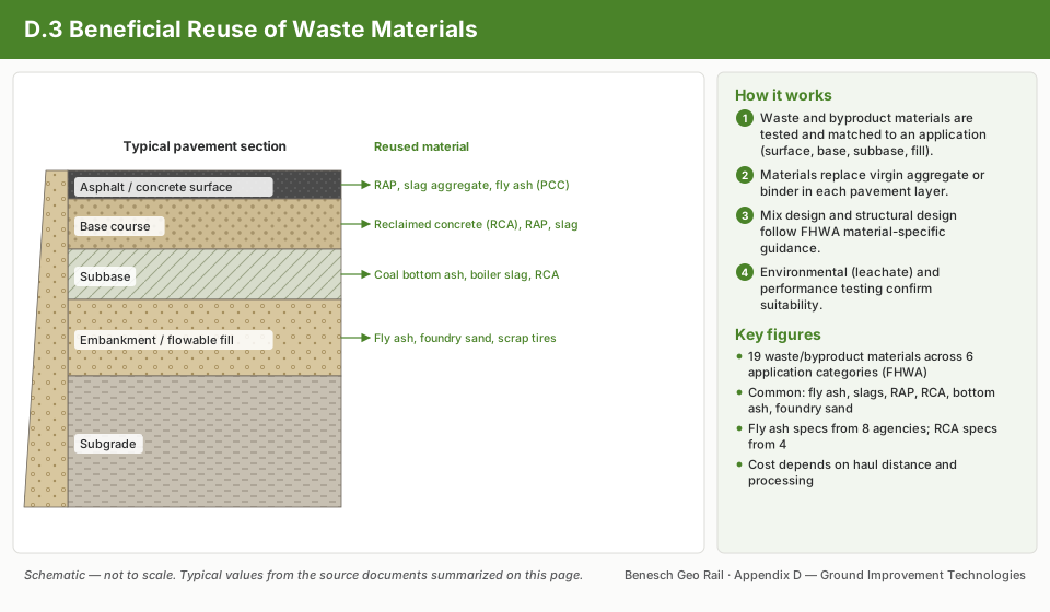
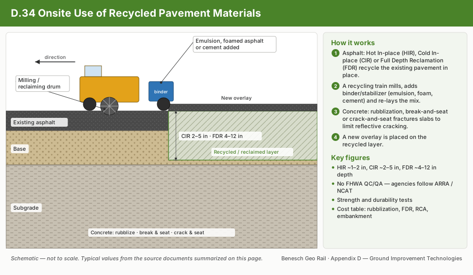
Chemical Stabilization of Subgrades and Bases schematic17.16.7Chemical Stabilization of Subgrades and BasesBio-Treatment for Subgrade Stabilization schematic17.16.2Bio-Treatment for Subgrade StabilizationMechanical Stabilization of Subgrades and Bases schematic17.16.31Mechanical Stabilization of Subgrades and BasesExcavation and Replacement schematic17.16.16Excavation and ReplacementBeneficial Reuse of Waste Materials schematic17.16.3Beneficial Reuse of Waste MaterialsOnsite Use of Recycled Pavement Materials schematic17.16.34Onsite Use of Recycled Pavement Materials

Case study: 17.17.3 Lime-treated local soil in a reinforced slope: choosing by total internalised cost (Look 2023), in §17.17 Case Studies.

Project management · Bull (2015)

Life-Cycle Selection Among No Treatment, In-Place Stabilization and Remove-and-Replace

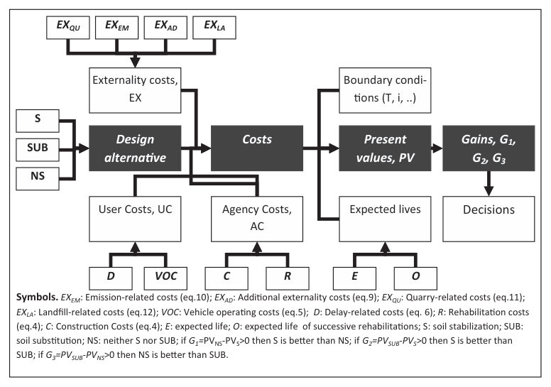
In Bull’s volume, Praticò, Saride and Puppala (Chapter 3) build a life-cycle cost model for choosing among three ways of treating a weak subgrade:

  • NS: leave the soil as it is.
  • S: stabilize it in place.
  • SUB: excavate and replace it.

Each alternative has an expected life that comes from its mechanical properties. Its present value sums three kinds of cost:

  • Agency costs: construction, rehabilitation and maintenance.
  • User costs: work-zone delay and vehicle operating costs.
  • Externality costs: emissions from hauling, quarrying and landfill.

Over an infinite horizon, where the first rehabilitation falls at year E and repeats every O years, the agency present value is:

PV = C + CRE × (1+i)−E / [1 − (1+i)−O]

The “gain” of one alternative over another is simply the difference in their present values.

The authors tested the model on two low-volume roads at a 4% discount rate. In the Italian case, a lime-treated CL subgrade was given a 20-year life against 15 years untreated. Stabilization beat substitution when stabilization was cheap. User costs were only about 1/50 of agency costs at those traffic levels. User gains turned negative once the treated alternative’s work zone lasted about 1.5 times as long as the untreated case. Stabilization paid at higher traffic. At very low traffic, remove-and-replace cost more than doing nothing. In the Texas case, lime–cement treatment turned a CH soil with 6.3% free swell into a non-swelling CL. Its unconfined strength rose from about 13 to 250 psi, and its resilient modulus from about 6 to 35 ksi.

For railroad work: the same three choices come up at most chronic subgrade sites:

  • NS: keep surfacing.
  • S: stabilize in place, by lime or cement treatment or by injection.
  • SUB: undercut and replace with subballast.

The perpetual-cycle factor shows how much each added year of life is worth. At 4%, (1.04)−15/[1 − (1.04)−15] = 1.25, while the same factor at 20 years is 0.84. So a treatment that stretches the maintenance cycle from 15 to 20 years cuts the present value of all future rehabilitation by about a third. Replace the highway user costs with train-delay and slow-order costs. Count the haul trips, quarried aggregate and disposed spoil or fouled ballast as externalities. Then test how the ranking changes with treatment cost and traffic (MGT), as the authors do.

Praticò, Saride and Puppala’s life-cycle model linking design alternatives, expected lives, agency, user and externality costs to present values and the “gain” indicators.
Figure 17-PM1. Praticò, Saride and Puppala’s life-cycle model linking design alternatives, expected lives, agency, user and externality costs to present values and the “gain” indicators. Source: Bull (2015), Figure 3.1.

Source: Bull, J. W. (ed.) (2015). Life Cycle Costing for the Analysis, Management and Maintenance of Civil Engineering Infrastructure. Dunbeath, Scotland: Whittles Publishing, pp. 66–77. Summarized and paraphrased; figures reproduced for internal reference. Full reference under Supplemental Sources.

17.8 Geosynthetic Reinforcement
17.8.1 Geotextile Filtration and Separation

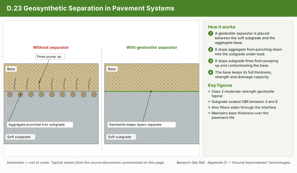
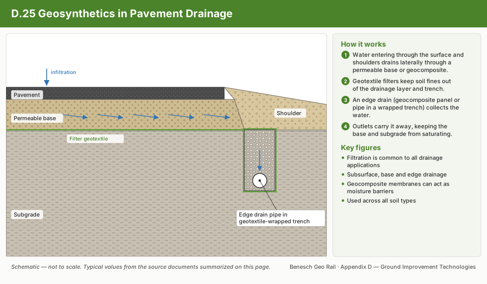
Geotextiles placed at subgrade/subballast and subgrade/subbase interfaces prevent fines migration (filtration) and maintain aggregate performance (separation). Key design criteria:

Apparent Opening Size (AOS) criterion:

AOS ≤ D85,soil    (retention criterion)

Permeability criterion:

kgeotextile ≥ ksoil    (permittivity criterion)

AREMA MRE Chapter 1 specifies minimum permittivity of 0.02 s⁻¹ for track subgrade geotextiles. NSR, CSXT, and BNSF all reference this criterion in their earthwork specifications.

Reference graphics

Geotextile placement, Kansas DOT
Geotextile Selection — Woven vs Nonwoven
Geotextile Design for Coastal Protection

Reference graphics · click to zoom

Geotextile Filter Design

Geotextiles and geomembranes under track: what the field record shows

Use a geotextile for what it can do.

  • It is poor at reinforcement. It needs large stretch to work, creeps, slips against ballast, and its openings enlarge as it stretches. Use geogrid for reinforcement.
  • Its main role is separation, with filtration of seepage and in-plane drainage as secondary roles.
  • It does not shed water from above.

Requirements.

  • Only nonwoven fabrics are acceptable.
  • AOS < D85 of the protected soil. For a gap-graded soil, base this on the fines fraction. For new ballast over an undercut surface, use the gradation of the fouling material and ignore the ballast-size particles.
  • High tensile, puncture, elongation, abrasion, chemical and UV resistance.
  • Proven resistance to clogging, and a thick mat where transmissivity is needed.

Nonwovens fine enough for silt, and especially clay, may not exist.

Placement.

  • At least 12 in. below the tie bottom, out of reach of tamping tines and undercutter chains.
  • On a smooth surface sloped to drain, with no equipment running on the fabric and minimal UV exposure.
  • Never in double layers, which create a slip plane.

Durability record.

  • On Norfolk Southern, fabric permeability fell 92% and transmissivity 85% within 15 months. Tensile strength fell 54% within 48 months.
  • At an AAR site near Caldwell, Texas, a clogged low-permittivity fabric trapped water, causing excess pore pressure and subgrade failure. It was believed to be the cause of a derailment.

“Undercut and add fabric” repairs often fail because the mud was not coming from the subgrade, or because the subgrade fines were too fine for the fabric. The book’s process is: diagnose the cause in the field and lab; compare geotextile and non-geotextile options; do an economic analysis; run a field trial; monitor and document. Only a properly graded, durable granular layer gives permanent separation and filtration (Chapter 2, §2.5.4).

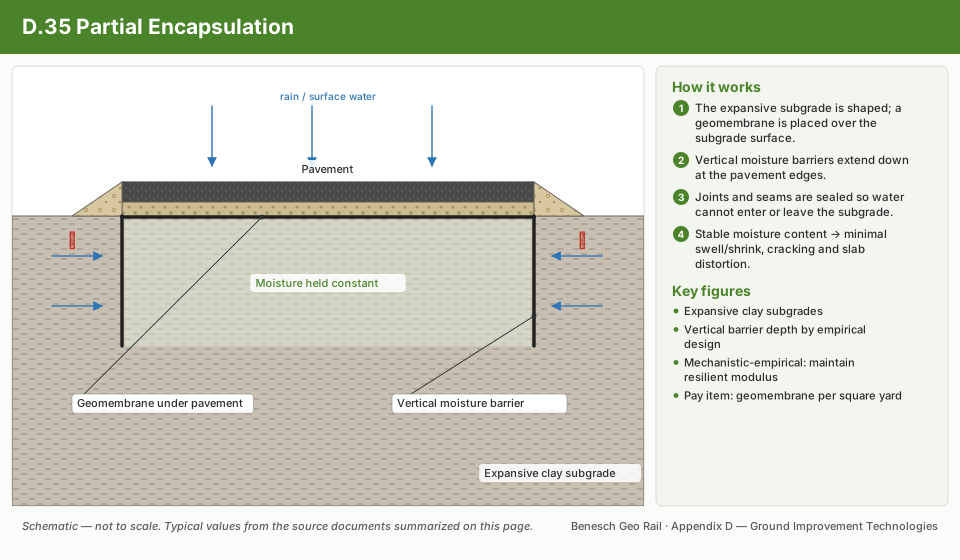
Geomembranes. Uses:

  • Blocking surface infiltration. Place the membrane between sand layers at least 2–4 in. thick, never against ballast, and drain the water off its top.
  • Keeping expansive soil from drying.
  • Cutting capillary rise in frost-susceptible embankments.
  • Forming a cut-off below the water table in cuts.

Hazards: water trapped beneath the membrane creates a slip surface, and holes or leaky seams concentrate flow and erode soil, which is worse than having no membrane. Most leaks are at seams, so require seam testing. A bitumen emulsion sprayed into a sand or subballast layer, which can be done behind an undercutter, is a cheaper alternative with the same trapped-water risk.

After Selig & Waters (1994), ch. 12. Full reference under Supplemental Sources.

17.8.2 Geogrid Reinforcement

Biaxial geogrids (ASTM D6637) placed at subgrade/subbase interface improve load distribution and reduce differential settlement. The Giroud-Han (2004) method for granular layer thickness over weak subgrade:

h = P / (Ap ⋅ ps) - 1KR ⋅ (1 + ε ⋅ h/√Ap)    (iterative; ft)

Where:

  • P = wheel load per wheel (lb)
  • A_p = contact area per wheel (in.²); for intermodal reach stacker: A_p ≈ 100 in.²
  • p_s = allowable subgrade stress = 3.2 × s_u for non-reinforced; 3.2 × s_u × TBR for reinforced
  • TBR = traffic benefit ratio (1.5–3.0 for biaxial geogrid)
  • K_R = load distribution factor (depends on h, A_p, and layer modular ratio)

For preliminary design, the simplified California chart method (USACE TM 5-818-8) is also acceptable when subgrade CBR and geogrid type are known.

Reference graphics

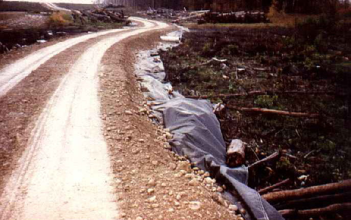
Geosynthetic-reinforced haul road
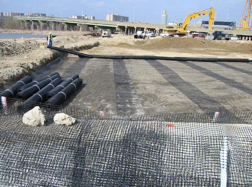
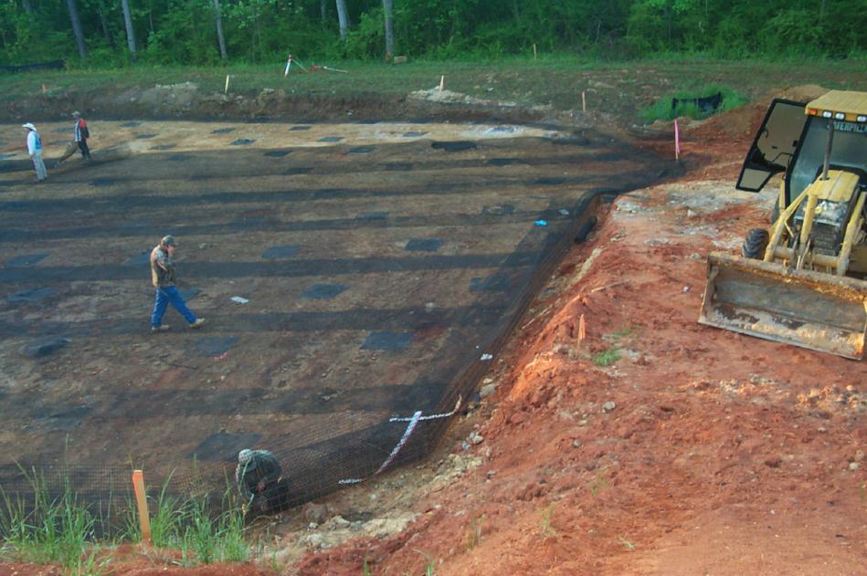
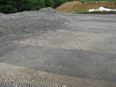
Geogrid placement on subgrade
Geosynthetic placement
17.8.3 Geosynthetic-Reinforced Load Transfer Platform (GRLT)

Over piled foundations or column-supported embankments (stone columns, rigid inclusions), a Geosynthetic-Reinforced Load Transfer Platform (GRLT) distributes track loads to column heads. GRLT design follows BS 8006:2010 or FHWA-HRT-17-097 (Giroud-Han approach):

Membrane tension in geosynthetic over column caps:

Tgeosynthetic = WT ⋅ s28 ⋅ δallow    (lb/ft)    (catenary approximation)

Where W_T = net soil weight transferred to geosynthetic (psf); s = clear span between column caps (ft); δ_allow = allowable deflection (in.); typically δ ≤ s/30 for railroad applications.

Reference graphics

Base geosynthetic layer over columns
Fill placement tensioning geosynthetic
Select fill placement over geosynthetic

Geotextiles in railway subgrades

  • Types: woven (two perpendicular fiber sets, strongly anisotropic) and non-woven (random fibers, isotropic); polypropylene or polyester; 0.016–0.12 in. thick; 2.1–10 oz/yd².
  • Functions: separation of granular layers, reinforcement of weak soil, filtration and drainage, and some frost protection. Most railway installations are simply separators between subballast and subgrade.
  • Placement: under the subballast, never directly under ballast. A geotextile does not spread load, so it must not be used as a reason to reduce ballast or subballast thickness. Railways that did so saw puncture of the fabric and loss of the crossfall.
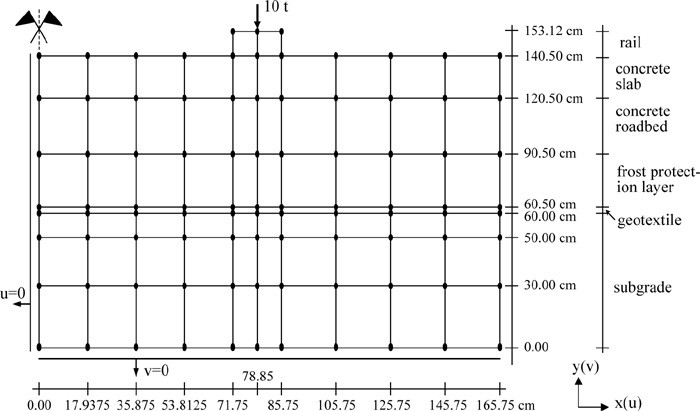
  • Benefit: a finite-element study found about a 10% reduction in stress at the top of subgrade (Figure 17-12). Maintenance savings were reported to repay the geotextile cost quickly.
  • Acceptance: verify tensile strength, elongation at failure, puncture and compressive strength, permeability and filtration against the soil before use. Filter criteria are in Chapter 2, §2.8.

Figures · click to zoom

Figure 17-12. Finite-element mesh for assessing the reinforcing effect of a geotextile in a railway subgrade. Profillidis Fig. 9.20.

After Profillidis (2014), §9.15, Fig. 9.20. Full reference under Supplemental Sources.

Geosynthetics, HMA underlayment and EPS: case histories

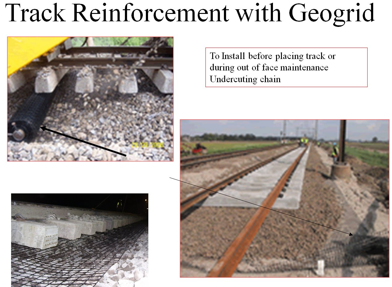
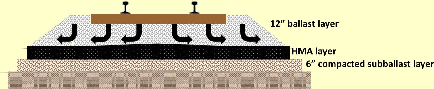
Geogrid can be placed before laying track or during out-of-face work with an undercutting chain. A hot-mix asphalt layer between 12 in. of ballast and 6 in. of compacted sub ballast spreads load and sheds water to the sides.

  • Rosetown Sub Mile 63.65: subgrade fines contaminated the ballast. Finger tests confirmed plastic fines, and bearing calculations sized the fix: excavate, place full-width woven geotextile, and backfill with clean granular fill.
  • Drummondville Sub Mile 42.7: decomposed corduroy and organic soil pumped mud. The fix was a shear-key trench along the shoulder backfilled with clean ballast (ideally with nonwoven geotextile), shoulders regraded to drain, and the trench left to drain ballast pockets toward the clay below.
  • Bala 47: woven geotextile placed beneath a lifted track panel at night within a possession window.
  • EPS lightweight fill (about $670/m³, or about $19/ft³, in 2016 dollars; about $600/m³ in 2012) reduces load on soft ground, but it can float in a flood unless ballasted and drained.

Figures · click to zoom

Figure 17-18. Geogrid reinforcement under the ties or by undercutting chain.
Figure 17-19. HMA underlayment between ballast and sub ballast, shedding water to the sides.
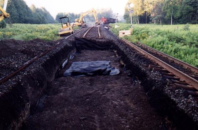
Figure 17-20. Full-width woven geotextile at Rosetown.
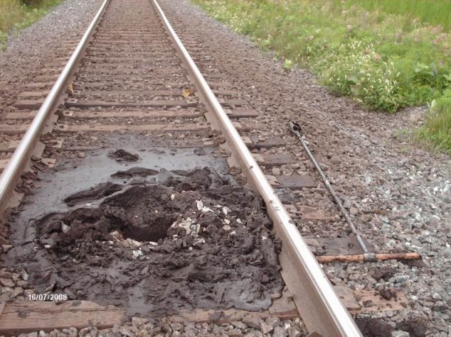
Figure 17-21. Organic mud pumping through ballast at Drummondville.
Figure 17-22. Track panel lifted for geotextile placement at Bala 47.
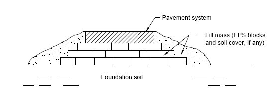
Figure 17-23. EPS block fill mass over soft foundation soil.
Figure 17-24. EPS blocks being placed.

After Geotechnology for Railroaders Program, Module 6.2; §03–05. Full reference under Supplemental Sources.

Geotextile handling under track

  • Limit sunlight exposure to 7 days from removal of the shipping cover to final placement.
  • Keep equipment off geotextile until it has at least 6 in. of sub-ballast or ballast cover.
  • Overlap at least 3 ft in both the longitudinal and transverse directions.
  • Direct surface drainage away from placed fabric to prevent contamination.

Inspection checks are in Chapter 15, Table 15-S1.

After UFC 4-860-01FA (2004), ch. 9, §4b. Full reference under Supplemental Sources.

Technology sheets for this method · see 17.16 Technology Library

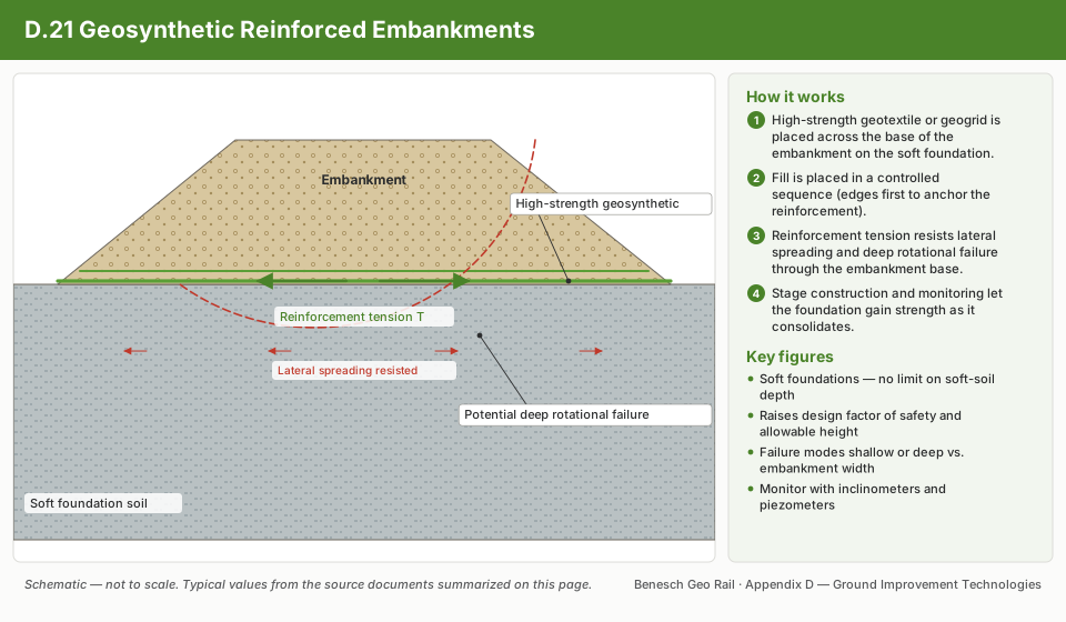
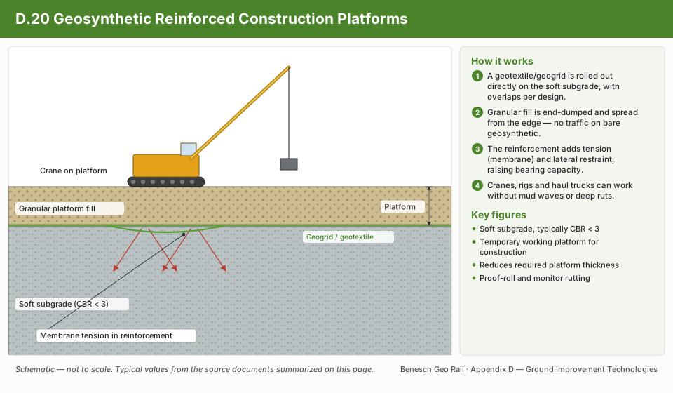
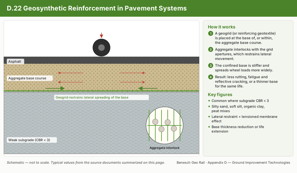
Geosynthetic Reinforced Embankments schematic17.16.21Geosynthetic Reinforced EmbankmentsGeosynthetic Reinforced Construction Platforms schematic17.16.20Geosynthetic Reinforced Construction PlatformsGeosynthetic Reinforcement in Pavement Systems schematic17.16.22Geosynthetic Reinforcement in Pavement SystemsGeosynthetic Separation in Pavement Systems schematic17.16.23Geosynthetic Separation in Pavement SystemsGeosynthetics in Pavement Drainage schematic17.16.25Geosynthetics in Pavement DrainageGeocell Confinement in Pavement Systems schematic17.16.19Geocell Confinement in Pavement SystemsFiber Reinforcement in Pavement Systems schematic17.16.17Fiber Reinforcement in Pavement SystemsGeoWEB schematic17.16.18GeoWEBGeosynthetics - GeoTerra schematic17.16.24Geosynthetics - GeoTerraPartial Encapsulation schematic17.16.35Partial Encapsulation

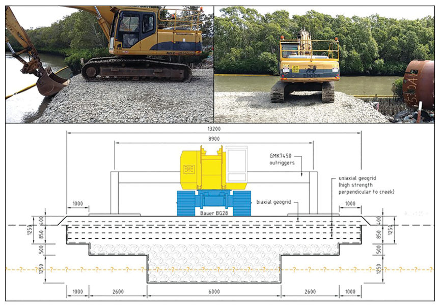
Case study: 17.17.4 Working platform at the edge of a creek, designed for slope stability (Look 2023), in §17.17 Case Studies.

17.9 Worked Examples

Worked Example 17-1: PVD Drain Spacing Design — CSXT Georgia Coastal Embankment

Project: CSXT mainline embankment widening, coastal Georgia. Soft CH clay, H = 30 ft. c_h = 0.012 ft²/day; c_v = 0.006 ft²/day. Target: U_total ≥ 90% in 120 days to allow next fill stage.

Step 1 — Vertical consolidation (Terzaghi):

Tv = cv ⋅ tHdr2 = 0.006 × 120(15)2 = 0.720225 = 0.0032

U_v ≈ 6.4% at T_v = 0.0032 (negligible; vertical drainage almost zero in 120 days for 30-ft layer).

Step 2 — Required radial consolidation (from combined equation):

1 - 0.90 = (1 - Ur)(1 - 0.064) ⇒ 0.10 = (1 - Ur)(0.936)
1 - Ur = 0.107 ⇒ Ur = 0.893

Step 3 — Required T_r:

0.107 = exp(-8 Trμ)
ln(0.107) = -8 Trμ ⇒ -2.235 = -8 Trμ ⇒ Tr = 2.235 μ8

Step 4 — Trial drain spacing (s = 5.0 ft, triangular grid):

d_e = 1.05 × 5.0 = 5.25 ft; d_w = 0.196 ft; ignore smear and resistance:

μ = ln(5.250.196) - 0.75 = ln(26.8) - 0.75 = 3.288 - 0.75 = 2.538
Tr = 2.235 × 2.5388 = 5.6748 = 0.709
t = Tr ⋅ de2ch = 0.709 × (5.25)20.012 = 19.530.012 = 1,628 days    (way too long)

Step 5 — Tighten spacing to s = 2.0 ft, triangular grid:

d_e = 1.05 × 2.0 = 2.10 ft; μ = ln(2.10/0.196) − 0.75 = ln(10.71) − 0.75 = 2.371 − 0.75 = 1.621

t = 0.709 × (2.10)20.012 = 0.709 × 4.410.012 = 3.1270.012 = 261 days    (still too long)

Step 6 — s = 1.5 ft, triangular grid:

d_e = 1.05 × 1.5 = 1.575 ft; μ = ln(1.575/0.196) − 0.75 = ln(8.035) − 0.75 = 2.084 − 0.75 = 1.334

t = 0.709 × (1.575)20.012 = 0.709 × 2.4810.012 = 1.7590.012 = 147 days

Step 7 — s = 1.25 ft triangular:

d_e = 1.05 × 1.25 = 1.3125 ft; μ = ln(1.3125/0.196) − 0.75 = ln(6.696) − 0.75 = 1.902 − 0.75 = 1.152

t = 0.709 × (1.3125)20.012 = 0.709 × 1.7230.012 = 1.2210.012 = 102 days < 120 days ✓

Recommendation: Install PVDs at 1.25-ft triangular grid spacing to achieve U_total ≥ 90% in approximately 102 days (within 120-day construction window). CSXT requires PVDs installed by displacement mandrel (static push, no vibration) to avoid disturbing soft clay structure. Piezometers at 3 depths to monitor dissipation; continue monitoring until U_r ≥ 90% confirmed before next fill stage.

Worked Example 17-2: Stone Column Design — BNSF Intermodal Yard, Gulf Coast

Project: BNSF Port Arthur container laydown area; CH clay subgrade, s_u = 450 psf; c_v = 0.005 ft²/day; H_clay = 18 ft. Applied stress from 4-high container stack: Δσ = 1,800 psf. Target: reduce post-improvement settlement to ≤ 6 in. (BNSF EI laydown area).

Step 1 — Untreated settlement estimate:

Sc,untreated = Cc H1 + e0 logσ'0 + Δσσ'0

σ'_0 = 1,100 psf (mid-layer); C_c = 0.45; e_0 = 1.20:

Sc = 0.45 × 181 + 1.20 log1,100 + 1,8001,100 = 8.12.20 × log(2.636) = 3.68 × 0.421 = 1.55 ft = 18.6 in.

Step 2 — Required improvement factor n₀:

Required: S_improved ≤ 6 in.; n₀ ≥ 18.6/6 = 3.1

Step 3 — Select stone column configuration:

Try D_c = 30 in. (2.5 ft), s_col = 5.0 ft square grid:

as = π (2.5)2 / 4(5.0)2 = 4.90925.0 = 0.196

Using Priebe (1995) with φ'_col = 40°, K_a = 0.217; simplified improvement factor estimate:

n0 ≈ 11 - as(1 - 11 + as Ka-1 (1 - 2νs)/(1 - νs))

For preliminary design, use empirical chart (Priebe 1995): a_s = 0.196, n₀ ≈ 2.5 (from chart, φ'_col = 40°).

Step 4 — Revised spacing:

Try D_c = 36 in. (3.0 ft), s_col = 5.0 ft: a_s = π(3.0)²/4/(25.0) = 7.069/25.0 = 0.283 → n₀ ≈ 3.2 (Priebe chart, a_s = 0.283)

Simproved = 18.63.2 = 5.8 in. ≤ 6 in. ✓

Recommendation: 36-in. diameter stone columns at 5-ft square grid, installed to H_clay = 18 ft. Crushed stone fill: 3/4-in. to 3-in. angular aggregate, φ'_col ≥ 40°. Load test (ASTM D1143) on one production column per 100 columns, minimum 5 tests. Settlement monitoring plate at each quadrant of stacking area to confirm performance. BNSF EI requires post-improvement CBR ≥ 8% at subgrade surface; verify by plate bearing test (ASTM D1196).

Worked Example 17-3: Lime Stabilization Design — CPKC Prairie Clay, Moose Jaw, SK

Project: CPKC MOW access road subgrade; CH clay (LL = 66, PL = 20, PI = 46); sulfate content = 850 ppm (acceptable for lime). γ_d,max = 93 pcf (Modified Proctor); w_opt = 22%. Target: PI_final < 12 for use as stable subgrade.

Step 1 — Lime content selection:

PI reduction rule: PI_final ≈ PI_initial − 5 × L_p

Target PI_final = 12: 12 = 46 − 5 × L_p → L_p = (46 − 12)/5 = 6.8% → Use 7% hydrated lime (rounding up)

Step 2 — Proctor mix design check:

Laboratory Proctor on lime-treated mix at L_p = 7%: γ_d,max,lime ≈ 88 pcf (typically 5–7 pcf reduction from lime addition); w_opt,lime ≈ 24% (moisture optimum increases with lime).

Step 3 — Expected strength gain (28 days):

For CH clay with 7% lime at 28 days: q_u,28 ≈ 90–130 psi (from laboratory trial mixes). Target q_u ≥ 50 psi per CPKC TS for stabilized subgrade.

Step 4 — Field specification:

  • Lime content: 7% by dry soil weight; hydrated lime (ASTM C977, Type S)
  • Mixing depth: 12 in. (top of subgrade)
  • Mellowing period: 24–48 hours before final compaction
  • Compaction: 98% Modified Proctor RC (CPKC TS); moisture −2% to +1% of w_opt
  • Curing: Protect from freezing for 3 days minimum (geotextile insulating blanket in autumn)
  • QC testing: pH ≥ 12.4 post-mixing (confirms adequate lime reaction); PI at 1 day and 7 days; q_u at 7 days and 28 days (ASTM D2166)

Sulfate verification: Retest sulfate content from each borrow area lot ≥ 500 yd³. If SO₄ > 2,000 ppm encountered, immediately switch to Type II/V cement at 5–6% binder content.

17.10 Representative Data Table
Table 17-4: Ground Improvement Performance Summary — Multi-Client Railroad Projects
ProjectRailroadSoft SoilMethodSpacing/GridImprovement FactorPre-Treat S_c (in.)Post-Treat S_c (in.)Performance Met?
Coastal GA EmbankmentCSXTCH clay, 35 ftPVDs @ 1.5-ft tri1.5 ftU_total = 90%N/A (time)120 daysYes
Port Arthur YardBNSFCH clay, 18 ftStone col., 36 in.@5 ftSquare 5 ftn₀ = 3.218.65.8Yes
Moose Jaw RoadCPKCCH clay, PI=467% lime, 12-in. depthN/API: 46→11N/API=11Yes
Winnipeg TerminalCNVarved clay, 25 ftDSM col., 24-in.@5 ftHex 5 ftn₀ = 2.814.25.1Yes
Willamette BridgeUPRRLoose sand, liq.DSM panels + cols3 ft gridFS_L: 0.67→1.35——Yes
NEC EmbankmentAmtrakSoft clay, 20 ftPVDs @ 1.25-ft tri1.25 ftU_total = 95%—75 daysYes
Atlanta Yard CLNSRCL clay, PI=225% lime, 12-in. depthN/API: 22→10N/API=10Yes
17.11 Figure Placeholders

Figure 17-1: Ground improvement method selection chart — applied stress vs. layer thickness for soft clay, showing PVD (staged), stone columns, DSM, and grouting zones.

Figure 17-2: PVD installation schematic — mandrel, drain card detail (a × b dimensions), smear zone d_s, equivalent drain diameter d_w, and influence zone d_e annotation.

Figure 17-3: U_r vs. time curves (Barron radial consolidation) for c_h = 0.012 ft²/day at drain spacings of 1.0, 1.25, 1.5, 2.0, and 3.0 ft (triangular grid). CSXT Georgia design point highlighted.

Figure 17-4: Priebe (1995) improvement factor chart — n₀ vs. a_s for φ'_col = 35°, 37.5°, 40°, 42°, 45°. BNSF Port Arthur case plotted at a_s = 0.283, n₀ = 3.2.

Figure 17-5: Stone column installation schematic — vibro-replacement wet process and dry process comparison, column grid plan view (square vs. triangular), and load transfer mechanism diagram.

Figure 17-6: DSM column cross-section — auger/mixing head, binder injection ports, column diameter range by system, and soil-cement micro-structure schematic.

Figure 17-7: Compaction grouting sequence — primary, secondary, and tertiary injection point grid; grout bulb growth schematic; vibration monitoring instrument location.

Figure 17-8: Lime stabilization PI reduction vs. lime content for typical CL and CH clays — laboratory data scatter with CPKC target PI < 12 line shown.

Figure 17-9: Geosynthetic-Reinforced Load Transfer Platform (GRLT) cross-section over stone column grid — geogrid layers, column caps, granular LTP, and track load distribution.

Figure 17-10: Staged embankment construction schedule — Stage 1 fill placement, PVD consolidation wait period, strength gain, Stage 2 fill, and settlement monitoring timeline with instrumentation triggers.

Reference graphics

Ground Improvement Methods
Stone column construction with vibro rigs
Cement-soil column auger and cement hopper
Proctor Compaction Test
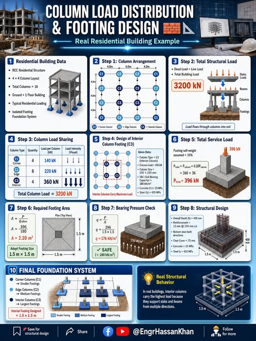
Column Load Distribution
17.12 Practical Recommendations
  1. Select the improvement method based on the governing constraint, not generic practice. For railroad applications, the governing constraint is almost always time (construction schedule), not cost. PVDs with surcharge are cost-effective but slow; DSM and stone columns are faster but more expensive. Always map the client's construction schedule against the consolidation time required for each method before recommending.
  2. Conduct a pre-improvement investigation parallel to improvement design. Ground improvement design requires additional data beyond standard investigation: c_h (from horizontal permeability tests or piezocone dissipation testing), sensitivity (from VST — Chapter 7), OCR profile (from consolidation test or CPTu — Chapters 7, 8, 12). Schedule these tests during the same mobilization as standard borings to avoid a second mobilization.
  3. Verify smear zone impact on PVD performance before finalizing spacing. In sensitive and structured clays (Amtrak NEC, CN Quebec), mandrel installation smears the horizontal permeability zone by a factor k_h/k_s of 3–8. Uncorrected Hansbo-Barron analysis that ignores smear will overestimate consolidation rate by 30–60%, leading to inadequate wait periods. Use the full μ formulation or correct from piezocone dissipation results.
  4. Install pre-construction and post-improvement plate bearing tests for stone column and DSM projects. Improvement factor n₀ is a design estimate. UPRR, BNSF, and CN all require at least one post-treatment plate bearing or pressuremeter test per 5,000 ft² of treated area to verify that the design improvement factor has been achieved in the field. Document pre-improvement and post-improvement data in the same GDR section for direct comparison.
  5. Do not specify lime treatment without sulfate testing. Ettringite swell from high-sulfate clays has caused major track heave failures on multiple Class I railroads. The roughly $28–55 cost (2016 dollars) of an ASTM D4327 sulfate test is trivial compared to remediation of failed lime stabilization. Test every distinct soil horizon and every new borrow area before specifying lime.
  6. Coordinate vibration exclusion zones with railroad operations before mobilization. Dynamic compaction and vibratory pile driving within 150–200 ft of active track require written authorization from the client's chief engineer, a pre-activity vibration baseline, continuous PPV monitoring during work, and a defined shutdown threshold (typically 0.5 in./s at rail). Failure to coordinate this before mobilization results in work stoppages and day-rate equipment charges. Obtain written approval from UPRR, BNSF, or CN engineering at least 30 days before activity.
  7. Provide a performance monitoring plan as a deliverable — not an afterthought. Ground improvement performance is verified by instrumentation: settlement plates, piezometers, inclinometers, and periodic plate bearing or vane shear tests. The monitoring plan, trigger levels, and reporting frequency should be finalized during design and included in the GDR. UPRR and BNSF expect electronic data transmittal to their infrastructure management systems weekly during active consolidation monitoring.
Project management · Miller (2009)

Precedence Logic, Lags and Effective-Workday Durations for Ground Improvement Sequencing

Miller describes the precedence diagramming method (PDM), in which boxes are activities and arrows are relationships. PDM allows four link types: finish-to-start (F-S), start-to-start (S-S), finish-to-finish (F-F) and start-to-finish (S-F). He considers F-S sufficient for almost every real situation and warns that the other three are seldom needed. A lag is a delay placed on a link. It is appropriate only for a true waiting period that uses no resources and is outside the manager’s control, such as shipping time. It should not be used to hide work, and because most software does not draw lags on the network, they show up only in the dates.

Two further points apply to duration estimates. First, the most common network flaw is building logic around limited resources; logic should assume unlimited resources, with resource conflicts resolved later during scheduling. Second, subject-matter experts usually estimate workload (hours of effort for an average performer), not duration. Duration is workload divided by the effective workday, the hours per day actually available to the activity: 48 hours ÷ 6 hours per day = 8 days. Where an estimate is uncertain, Miller uses a PERT weighted average, (optimistic + 4 × most likely + pessimistic) ÷ 6; with 6, 10 and 20 days the result is about 11 days.

For railroad work:

  • Do not model a surcharge or PVD consolidation hold as a lag. It is a geotechnical hold point with an exit criterion (settlement rate or excess pore pressure from the monitoring program), so show it as a visible activity whose duration is the design estimate, with a separate “geotechnical release” milestone.
  • Lags suit genuine passive waiting periods, such as cure time before coring cement-treated or deep-mixed soil, or delivery of geosynthetics and drain material after approval of submittals.
  • S-S links with a lag describe production that follows behind other production: test-column verification or QC coring can start a set number of days after stone column or DSM installation starts, without waiting for it to finish.
  • For work under track protection, the effective workday is the authorized window minus time to set up protection, travel, and clear the track. Estimate rig or crew workload in hours and divide by that effective figure, not by the nominal shift length.

Source: Miller, D. P. (2009). Building a Project Work Breakdown Structure: Visualizing Objectives, Deliverables, Activities, and Schedules. ESI International Project Management Series. Boca Raton, FL: Auerbach Publications (CRC Press, Taylor & Francis Group), pp. 72–75, 105–109. Summarized and paraphrased. Full reference under Supplemental Sources.

Project management · Kelly et al. (2004)

Paired Comparison and Weighted Scoring for Option Selection

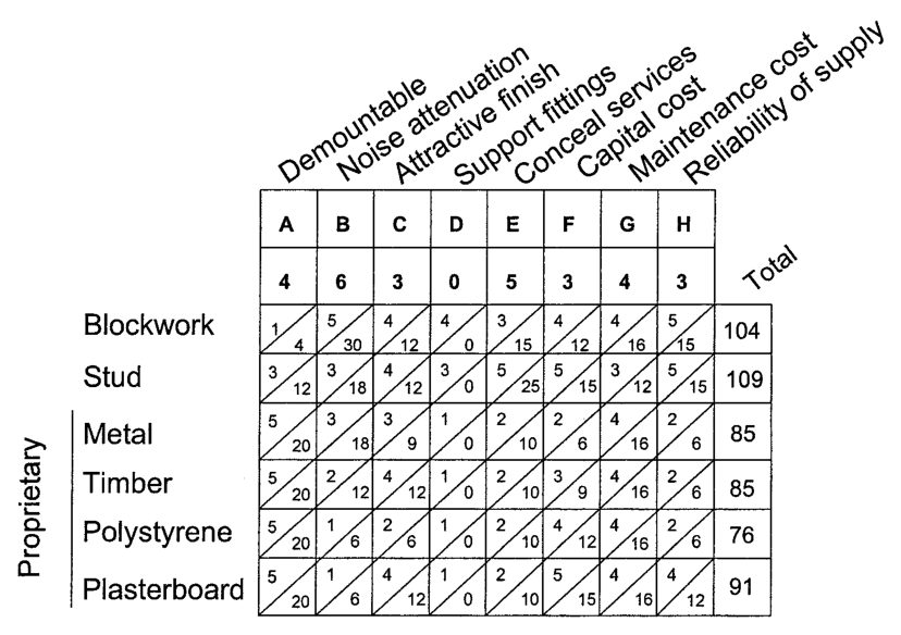
Kelly, Male and Graham recommend weighting and scoring when several technically feasible options compete and none is clearly best. The first step is to agree on the criteria. Correlated criteria should be avoided because they count the same attribute twice; their example is that ease of cleaning and cost of cleaning should not both be used. Weights then come from a paired comparison. Each criterion is compared with every other, the more important of each pair is recorded, and each criterion’s number of “wins” becomes its weight. Each option is scored 1–5 against each criterion. Score is multiplied by weight and the products are summed. Sensitivity checks, made by changing a few weights and scores, show whether the ranking is robust.

Their worked example compares internal partitions for a building that is reorganized every two to six years. Eight criteria (demountability, noise attenuation, finish, support of fittings, concealing services, capital cost, maintenance cost and reliability of supply) received weights of 4, 6, 3, 0, 5, 3, 4 and 3. Stud-and-board partitions totaled 109 and plastered blockwork 104, while the proprietary systems scored 76–91, mainly because noise attenuation carried the highest weight. The authors say the result should prompt a second look rather than be accepted mechanically. Any preferred option must still be technically feasible, economically viable, functionally suitable and acceptable to the client.
For railroad work: The method suits ground improvement and subgrade remediation choices, such as undercut-and-replace versus geogrid-reinforced subballast versus lime or cement stabilization versus deep soil mixing. Typical criteria are track outage required, ability to work from the track or the right-of-way, settlement performance under the design traffic in MGT, construction risk in the expected soils, capital cost, maintenance demand and supply-chain or contractor availability. Derive the weights with the railroad’s engineering and operations staff in the room, because operations typically values outage time very differently from engineering. Keep capital cost as one weighted criterion, or compare it separately on a whole-life basis, and show the sensitivity run in the report so the choice can be audited.

Paired-comparison grid in which each criterion is compared with every other, and the count of wins becomes the criterion weight.
Figure 17-PM2. Paired-comparison grid in which each criterion is compared with every other, and the count of wins becomes the criterion weight. Source: Kelly et al. (2004), Fig. A1.15.

Source: Kelly, J., Male, S. and Graham, D. (2004). Value Management of Construction Projects. Oxford: Blackwell Science, pp. 75–77, 308–310. Summarized and paraphrased; figures reproduced for internal reference. Full reference under Supplemental Sources.

Project management · ASCE (2013)

Prescriptive versus Performance Specifications for Ground Improvement

The ASCE Committee on Specifications defines two basic types of specification.

  • A prescriptive specification is a recipe. It names the materials, procedures and workmanship. If the contractor follows the recipe and the result falls short, the engineer is responsible.
  • A performance specification describes the end result and leaves products, equipment and techniques to the contractor.

A performance specification has three requirements:

  1. the end result must be described completely;
  2. it must be verifiable by straightforward testing or inspection with detailed acceptance criteria;
  3. the bidding period may need to be longer, because bidders may have to do development work before pricing.

The guide compares the two types as follows:

  • Bidding: easier under prescriptive specifications.
  • Innovation: favors performance specifications.
  • Design control: stays with the engineer under prescriptive specifications.
  • Cost: performance specifications usually cost less on complex work and make little difference on simple work.
  • Testing: prescriptive work needs more testing as it is placed, while performance work needs more testing of the finished product.

Prescriptive specifications fit where the end result cannot be fully defined or where loss of design control is unacceptable. Performance specifications fit where end-result specification is normal practice, or where the contractor’s ingenuity is wanted. The two can be combined, as with concrete specified by both strength and mix limits, but they must not conflict on the same product or activity.

For “or equal” clauses, list the salient characteristics that will be used to judge equality. Read every reference standard before citing it, because standards contain options and may conflict with one another. Do not over-specify. Each tighter quality level or tolerance adds cost.

For railroad work: Ground improvement suits a performance or hybrid approach, because specialty contractors own the equipment and know-how. A deep soil mixing or grouting GSP for an embankment or subgrade might specify:

  • minimum unconfined strength and coefficient-of-variation targets, from wet-grab or core testing at stated frequencies;
  • column geometry and overlap;
  • allowable heave or ground and track movement, monitored against track-geometry limits;
  • the mix design, test columns and QC records as contractor submittals.

Avoid also fixing the binder dosage and mixing energy unless the railroad accepts responsibility for the result. Stone columns and PVDs are often specified prescriptively (spacing, length, material). In that case acceptance should be based on installation records, and settlement performance should not be made a separate contractual guarantee unless the design responsibility is transferred clearly.

Source: ASCE Construction Institute Committee on Specifications (L. Eckersley, Chair) (2013). Preparation of Construction Specifications for Civil Projects. Reston, VA: American Society of Civil Engineers, pp. 14–22. Summarized and paraphrased. Full reference under Supplemental Sources.

Project management · Sullivan et al. (2015)

Breakeven Analysis: How Often Must a Problem Recur Before Improvement Pays?

Sullivan et al. use breakeven analysis when the choice between two alternatives turns mainly on one uncertain factor. Write the equivalent worth (PW or annual worth) of each alternative as a function of that factor, set the two expressions equal, and solve for the factor. If the best estimate of the factor lies above the breakeven value, one alternative wins; if below, the other does. The method works the same way for a single project: set its equivalent worth to zero and solve for the factor.

Factors commonly tested this way are annual expenses, interest rate, service life, and hours of use. In their examples, a hybrid car beats a conventional car only above a fuel price of $3.64/gal. Three motors trade places at 1,694 and 4,389 operating hours per year. In each case the analysis gives the decision-maker one number to argue about instead of a whole cash-flow table.

For railroad work: the classic case is ground improvement or undercutting compared with continued spot maintenance at a chronic soft subgrade or mud spot. The uncertain factor is how many maintenance interventions a year the location really needs. Each intervention includes surfacing, ballast, flagging, and the train-delay cost of the slow order that follows. As an illustration only, with inputs chosen for the example:

  • Permanent fix: $600,000 first cost, 25-year life, 7% discount rate. Its equivalent annual cost is $600,000 × (A/P, 7%, 25) = $600,000 × 0.0858 = $51,500/yr.
  • Each maintenance intervention: $12,000 all-in.
  • Breakeven: $51,500 / $12,000 = about 4.3 interventions per year, ignoring the small residual maintenance after the fix.

If track inspection records show the spot being surfaced six times a year, the fix is justified. If it is surfaced twice a year, it is not, unless safety risk or capacity value changes the picture. Two other breakeven tests are useful: the service life the improvement must achieve, and the first cost at which it stops paying. Present these breakeven values to the client rather than a single net present worth, because they show plainly which input the decision depends on. They also show which records to check, such as maintenance-of-way work orders and slow-order logs.

Source: Sullivan, W. G., Wicks, E. M. and Koelling, C. P. (2015). Engineering Economy, 16th ed. Upper Saddle River, NJ: Pearson, pp. 476–482. Summarized and paraphrased. Full reference under Supplemental Sources.

17.13 Ground Improvement Checklist

Checklist · Part VII · Stabilization Methods

Ground Improvement Checklist

Investigation Phase (Pre-Design)0 of 6
Design Phase0 of 8
Construction Phase0 of 6
Deliverable Phase0 of 5

Levy (2007) describes how a contractor builds a formal Construction Quality Control Plan (CQCP). A qualified CQCP manager owns the plan in the same way a safety director owns the safety program. The plan should include, at a minimum, an organization chart locating the CQCP manager, proposed personnel, designated authorities and their duties, operating procedures for inspections, tests and documentation, a subcontractor and vendor rating system, help in selecting quality-oriented subcontractors, training for field staff, and field inspection report forms.

The core tool is the inspection checklist: a short, numbered list of the quality points for one work type, signed and dated by the inspector. Levy’s concrete placement checklist, for example, runs from approved shop drawings on site and the correct strength ordered, through form and rebar approval, testing requirements (slump, number of cylinders, temperature), vibration, curing, and hot- or cold-weather protection. Similar lists can be prepared for every trade with help from an engineer or a qualified subcontractor. Checklists serve as a guide for less experienced supervisors and also signal that quality matters; copies can be given to the subcontractor to document compliance or deficiencies.

His inspection tips: check quality on every walkthrough and at least weekly; notify the subcontractor promptly of unacceptable work and set a date for correction, then verify it; if poor work continues, bring the subcontractor’s owner or the manufacturer’s representative to the site and confirm the meeting in writing; and walk the work for a punch list before a subcontractor demobilizes.

For railroad work: Ground improvement under or beside track lends itself to this method because acceptance depends on records produced as the work is done. A checklist for each technique (stone columns, jet grouting, compaction grouting, deep soil mixing, PVDs, geosynthetic placement) might cover approved submittal and mix design on site, layout against track stationing and clearance envelopes, installation parameters logged per element (depth, pressure, volume, time), spoil and heave observations, track surface monitoring during work near live track, sampling and testing frequency, and nonconformance actions. Signed checklists, combined with the element logs, give the railroad a defensible basis for accepting work that cannot be seen once it is installed.

Source: Levy, S. M. (2007). Project Management in Construction, 5th ed. New York: McGraw-Hill, pp. 220–227. Summarized and paraphrased. Full reference under Supplemental Sources.

Ticks are saved in this browser.
Plain text version

Investigation Phase (Pre-Design)

  • [ ] Confirm soft layer depth, thickness, and lateral extent from boring/CPTu data
  • [ ] Obtain c_v and c_h from consolidation tests and/or piezocone dissipation tests
  • [ ] Measure s_u profile (VST or CPTu N_kt method) to determine staged loading feasibility
  • [ ] Test sulfate content (ASTM D4327) at all sites where lime or cement stabilization is planned
  • [ ] Evaluate sensitivity (S_t = s_u / s_u,remolded) to assess disturbance risk from installation
  • [ ] Confirm access constraints (setback from track, overhead clearance, crane swing radius)

Design Phase

  • [ ] Select improvement method per Table 17-1 client standards and schedule constraint
  • [ ] For PVDs: compute d_e, μ (full formulation), T_r required; verify drain discharge capacity q_w
  • [ ] For stone columns: compute a_s, n₀ (Priebe); verify composite bearing capacity
  • [ ] For DSM: select binder type; set field q_u target ≥ 4× design q_u (f_lab = 0.25)
  • [ ] For lime/cement: run laboratory trial mixes at 4%, 6%, 8% binder; confirm target PI or q_u
  • [ ] For geosynthetics: verify AOS criterion for filtration; specify permittivity per AREMA Ch. 1
  • [ ] Prepare staged loading schedule with FS_slope ≥ 1.3 at each stage (see Chapter 13)
  • [ ] Define performance monitoring instrumentation plan (type, location, frequency, trigger levels)

Construction Phase

  • [ ] Verify mandrel type and size (PVD); document mandrel dimensions for smear zone estimate
  • [ ] Confirm as-installed drain/column locations vs. design grid; document deviations > 6 in.
  • [ ] Monitor piezometer responses and compare to predicted dissipation curves during wait period
  • [ ] Perform QC strength/bearing tests (Table 17-3 criteria) after improvement and before loading
  • [ ] Document any anomalous grout takes (grouting), column refusals (stone columns), or auger torque spikes (DSM)
  • [ ] Maintain vibration monitoring log for all activities within client exclusion zone

Deliverable Phase

  • [ ] Include improvement design calculation in GDR appendix (PVD spacing, stone column a_s/n₀, etc.)
  • [ ] Provide as-built drain/column layout plan
  • [ ] Provide performance monitoring data summary (piezometer, settlement plate, strength tests)
  • [ ] Compare post-improvement performance to design targets; note any deficiencies
  • [ ] Transmit monitoring data to client's infrastructure management system in required format
Project management · Levy (2007)

Construction Quality Control Plans and the Inspection Checklist Method

Levy (2007) describes how a contractor builds a formal Construction Quality Control Plan (CQCP). A qualified CQCP manager owns the plan in the same way a safety director owns the safety program. The plan should include, at a minimum, an organization chart locating the CQCP manager, proposed personnel, designated authorities and their duties, operating procedures for inspections, tests and documentation, a subcontractor and vendor rating system, help in selecting quality-oriented subcontractors, training for field staff, and field inspection report forms.

The core tool is the inspection checklist: a short, numbered list of the quality points for one work type, signed and dated by the inspector. Levy’s concrete placement checklist, for example, runs from approved shop drawings on site and the correct strength ordered, through form and rebar approval, testing requirements (slump, number of cylinders, temperature), vibration, curing, and hot- or cold-weather protection. Similar lists can be prepared for every trade with help from an engineer or a qualified subcontractor. Checklists serve as a guide for less experienced supervisors and also signal that quality matters; copies can be given to the subcontractor to document compliance or deficiencies.

His inspection tips: check quality on every walkthrough and at least weekly; notify the subcontractor promptly of unacceptable work and set a date for correction, then verify it; if poor work continues, bring the subcontractor’s owner or the manufacturer’s representative to the site and confirm the meeting in writing; and walk the work for a punch list before a subcontractor demobilizes.

For railroad work: Ground improvement under or beside track lends itself to this method because acceptance depends on records produced as the work is done. A checklist for each technique (stone columns, jet grouting, compaction grouting, deep soil mixing, PVDs, geosynthetic placement) might cover approved submittal and mix design on site, layout against track stationing and clearance envelopes, installation parameters logged per element (depth, pressure, volume, time), spoil and heave observations, track surface monitoring during work near live track, sampling and testing frequency, and nonconformance actions. Signed checklists, combined with the element logs, give the railroad a defensible basis for accepting work that cannot be seen once it is installed.

Source: Levy, S. M. (2007). Project Management in Construction, 5th ed. New York: McGraw-Hill, pp. 220–227. Summarized and paraphrased. Full reference under Supplemental Sources.

17.14 Practice Questions

Question 11-1: A CSXT coastal site has c_h = 0.015 ft²/day and soft clay layer H = 40 ft. PVDs are installed at s = 1.5 ft triangular grid (d_e = 1.575 ft; d_w = 0.196 ft). Compute U_r after 90 days (ignore smear and well resistance; ignore vertical consolidation for this problem).

Answer 11-1:

μ = ln(1.5750.196) - 0.75 = ln(8.035) - 0.75 = 2.084 - 0.75 = 1.334
Tr = ch ⋅ tde2 = 0.015 × 90(1.575)2 = 1.352.481 = 0.544
Ur = 1 - exp(-8 × 0.5441.334) = 1 - exp(-3.264) = 1 - 0.038 = 0.962 = 96.2%

U_r = 96% far exceeds the 90% target — the 1.5-ft spacing is conservative. A 1.75-ft spacing would also achieve 90% within 90 days, reducing PVD quantities approximately 36%.

Question 11-2: A BNSF site has CH clay with s_u = 400 psf and proposes stone columns D_c = 30 in. at 6.0-ft square grid. Calculate a_s and estimate n₀ using the Priebe simplified approximation (assume φ'_col = 40°). If untreated S_c = 15 in., what is the post-improvement settlement?

Answer 11-2:

as = π (2.5)2/4(6.0)2 = 4.90936.0 = 0.136

From Priebe (1995) chart or formula with φ'_col = 40° and a_s = 0.136: n₀ ≈ 2.1

Simproved = 15 in.2.1 = 7.1 in.

This exceeds BNSF's 6-in. target. Reduce spacing to 5.5 ft square: a_s = π(2.5)²/4/(30.25) = 0.162; n₀ ≈ 2.4; S_improved = 15/2.4 = 6.25 in. — still marginally over. Try 5.0-ft spacing: a_s = 0.196; n₀ ≈ 2.7; S_improved = 15/2.7 = 5.6 in. ≤ 6 in. ✓ Recommend 30-in. columns at 5.0-ft square grid.

Question 11-3: A CPKC site has CH clay with PI = 52 and sulfate content = 1,200 ppm. What lime content is needed to achieve PI_final = 12? Is sulfate a concern?

Answer 11-3:

Lp = PIi - PIf5 = 52 - 125 = 405 = 8.0%
  • Sulfate = 1,200 ppm < 2,000 ppm threshold → Lime treatment is acceptable. However, CPKC TS requires re-testing each lot ≥ 500 yd³ during construction. If any sample exceeds 2,000 ppm, switch to 5–6% Type II Portland cement (freeze-thaw durable) per CPKC TS sulfate procedure.
  • Specified lime: 8.0% Ca(OH)₂ by dry soil weight, ASTM C977 Type S.

Question 11-4: A UPRR embankment compaction specification requires 95% Modified Proctor on CL fill. Laboratory Proctor gives γ_d,max = 105 pcf at w_opt = 16%. A nuclear density gauge reading shows γ_d,field = 99.5 pcf at w = 18%. Is the fill acceptable?

Answer 11-4:

RC = 99.5105 × 100% = 94.8%

RC = 94.8% < 95% minimum → Not acceptable. The fill is also 2% above optimum moisture (+2% over w_opt = 16%). The wet condition reduces shear strength and increases settlement potential. Required action: scarify and dry back to w_opt ± 2% (14–18%); re-compact; re-test. For UPRR intermodal yard applications, moisture must also fall within −2% to +2% of w_opt; the current reading at w = 18% (exactly at +2%) is at the limit — additional passes with padfoot drum recommended before accepting.

Question 11-5: A DSM ground improvement program at an Amtrak NEC site targets q_u,field = 75 psi. What laboratory design strength should be specified, and what is the expected composite modulus E_composite if a_DSM = 0.25 and E_soil = 500 psi for the soft clay?

Answer 11-5:

  • Laboratory design strength using flab = 0.25: q_u,lab = q_u,field / f_lab = 75 / 0.25 = 300 psi (laboratory target)
  • E_DSM = 300 × q_u,field = 300 × 75 = 22,500 psi (using E_DSM = 300 × q_u,field, midpoint of 150–500 range)
  • Composite modulus:
  • Settlement reduction factor: E_composite/E_soil = 6,000/500 = 12× (substantial improvement)
  • Verify: post-improvement settlement S_improved = S_untreated/12. If untreated S = 3 in. (typical NEC soft clay), S_improved ≈ 0.25 in. — well within Amtrak's 0.50-in. NEC Class 7 track tolerance.
17.15 Cross-References
TopicRefer To
Laboratory consolidation parameters (c_v, C_c, e₀)Chapter 10, Sections 10.8–10.9
Settlement analysis — untreated and surchargeChapter 12, Sections 12.4–12.8
Slope stability — staged embankment loadingChapter 13, Section 13.6
Seismic liquefaction — DSM and stone column mitigationChapter 14, Section 14.7
Bearing capacity of improved groundChapter 11, Sections 11.3–11.4
Subgrade improvement for pavementChapter 18, Sections 18.6–18.7
Compaction testing — nuclear gauge, sand coneChapter 15, Sections 15.1–15.2
Geotechnical Special Provisions — ground improvementAppendix C
Monitoring instrumentation — settlement plates, piezometersChapter 15, Section 15.5

End of Chapter 17 — Ground Improvement Methods

17.16 Ground Improvement Technology Library

Sections 17.2 through 17.8 describe how each family of ground improvement works and how it is designed for railway loading. This library carries the supporting technology sheets: 45 techniques, numbered 17.16.1–17.16.45 in alphabetical order and grouped below by category. Each sheet opens with a how-it-works schematic and key figures, followed by its fact sheet, design guidance, QC/QA, specifications, cost information and case histories. Use the Previous / Next buttons at the bottom of each sheet to step through the library in order.

The sheets most relevant to each method are also linked at the end of Sections 17.2–17.8. Soil nailing, MSE walls and deep foundation sheets support Chapter 16 — Retaining Structures and Chapter 11 — Bearing Capacity.

Section 17.16 · Selection guide

Choosing a technology for a railway problem

Find the problem on the cross-section, read the section that explains the method, then open the technology sheets to compare options.

8Railway problems
35Technology sheets
Railway cross-section showing where each of the eight ground problems occurs Soft clayLoose sandBedrock Cut slopeStockpileEmbankment fill 1234 5678
1Locate the problem on the section
2Read the method in the chapter
3Compare the technology sheets
1
Soft clay under embankment

Soft, compressible clay under new or widened embankment

Drain, preload or support on columns
Technology sheets 6
17.16.36Prefabricated Vertical Drains and Fill Preloading17.16.43Vacuum Preloading with and without Prefabricated Vertical Drains17.16.8Column-Supported Embankments17.16.9Combined Soil Stabilization with Vertical Columns17.16.13Deep Mixing Methods17.16.26Geotextile Encased Columns
2
Loose sand or silty sand

Loose sand or silty sand — settlement or liquefaction

Densify or replace with columns
Technology sheets 6
17.16.45Vibrocompaction17.16.12Deep Dynamic Compaction17.16.37Rapid Impact Compaction17.16.4Blasting Densification17.16.1Aggregate Columns17.16.38Sand Compaction Piles
3
Weak or pumping subgrade

Weak or pumping subgrade under track, yard or access road

Stabilize, separate and reinforce
Technology sheets 6
17.16.7Chemical Stabilization of Subgrades and Bases17.16.31Mechanical Stabilization of Subgrades and Bases17.16.2Bio-Treatment for Subgrade Stabilization17.16.16Excavation and Replacement17.16.21Geosynthetic Reinforced Embankments17.16.23Geosynthetic Separation in Pavement Systems
4
Voids, sinkholes, lost backfill

Voids, sinkholes, abandoned mines or culvert backfill loss

Fill and densify by grouting
Read first
Technology sheets 4
17.16.10Compaction Grouting17.16.5Bulk-Infill Grouting17.16.6Chemical Grouting & Injection Systems17.16.30Jet Grouting
5
Cut or embankment slope instability
Nail, retain or reinforce
Technology sheets 6
17.16.14Drilled-Grouted and Hollow Bar Soil Nailing17.16.39Screw-in Soil Nailing17.16.40Shoot-in Soil Nailing17.16.32Mechanically Stabilized Earth Wall System17.16.41Shored Mechanically Stabilized Earth Wall System17.16.1Aggregate Columns
6
Foundations near live track

Foundations near live track / limited headroom

Small-footprint deep foundations
Technology sheets 4
17.16.33Micropiles17.16.27Helical Pile17.16.11Continuous Flight Auger Piles17.16.30Jet Grouting
7
Compaction QA & fill acceptance
Compact and verify
Technology sheets 3
17.16.29Intelligent Compaction17.16.42Traditional Compaction17.16.28High-Energy Impact Rollers
8
Reuse of on-site or recycled materials
Reuse instead of import
Technology sheets 3
17.16.3Beneficial Reuse of Waste Materials17.16.34Onsite Use of Recycled Pavement Materials17.16.16Excavation and Replacement

Click a number on the cross-section to jump to its card. Some technologies, such as aggregate columns, jet grouting, and excavation and replacement, serve more than one problem. Technology sheets open on dirtbert.com.

Open the selection guide on its own page (for printing) →

Full table: choosing a technology for a railway problem

Railway problemWhere the method is discussedTechnology sheets
Soft, compressible clay under new or widened embankment17.3 PVDs / preloading; 17.4–17.5 columns17.16.36 Prefabricated Vertical Drains and Fill Preloading
17.16.43 Vacuum Preloading with and without Prefabricated Vertical Drains
17.16.8 Column-Supported Embankments
17.16.9 Combined Soil Stabilization with Vertical Columns
17.16.13 Deep Mixing Methods
17.16.26 Geotextile Encased Columns
Loose sand or silty sand — settlement or liquefaction17.2 densification; 17.4 stone columns17.16.45 Vibrocompaction
17.16.12 Deep Dynamic Compaction
17.16.37 Rapid Impact Compaction
17.16.4 Blasting Densification
17.16.1 Aggregate Columns
17.16.38 Sand Compaction Piles
Weak or pumping subgrade under track, yard or access road17.7 stabilization; 17.8 geosynthetics17.16.7 Chemical Stabilization of Subgrades and Bases
17.16.31 Mechanical Stabilization of Subgrades and Bases
17.16.2 Bio-Treatment for Subgrade Stabilization
17.16.16 Excavation and Replacement
17.16.21 Geosynthetic Reinforced Embankments
17.16.23 Geosynthetic Separation in Pavement Systems
Voids, sinkholes, abandoned mines or culvert backfill loss17.6 grouting17.16.10 Compaction Grouting
17.16.5 Bulk-Infill Grouting
17.16.6 Chemical Grouting & Injection Systems
17.16.30 Jet Grouting
Cut slope or embankment slope instabilityCh 13 slope stability; Ch 16 retaining structures17.16.14 Drilled-Grouted and Hollow Bar Soil Nailing
17.16.39 Screw-in Soil Nailing
17.16.40 Shoot-in Soil Nailing
17.16.32 Mechanically Stabilized Earth Wall System
17.16.41 Shored Mechanically Stabilized Earth Wall System
17.16.1 Aggregate Columns
Foundations near live track / limited headroomCh 11 bearing capacity17.16.33 Micropiles
17.16.27 Helical Pile
17.16.11 Continuous Flight Auger Piles
17.16.30 Jet Grouting
Compaction QA and fill acceptance17.2 compaction; Ch 15 monitoring17.16.29 Intelligent Compaction
17.16.42 Traditional Compaction
17.16.28 High-Energy Impact Rollers
Reuse of on-site or recycled materials17.7 stabilization17.16.3 Beneficial Reuse of Waste Materials
17.16.34 Onsite Use of Recycled Pavement Materials
17.16.16 Excavation and Replacement

Vertical Columns & Deep Mixing (7)

Aggregate Columns schematic17.16.1Aggregate ColumnsColumn-Supported Embankments schematic17.16.8Column-Supported EmbankmentsCombined Soil Stabilization with Vertical Columns schematic17.16.9Combined Soil Stabilization with Vertical ColumnsDeep Mixing Methods schematic17.16.13Deep Mixing MethodsGeotextile Encased Columns schematic17.16.26Geotextile Encased ColumnsSand Compaction Piles schematic17.16.38Sand Compaction PilesVibro-Concrete Columns schematic17.16.44Vibro-Concrete Columns

Subgrade & Base Stabilization (3)

Bio-Treatment for Subgrade Stabilization schematic17.16.2Bio-Treatment for Subgrade StabilizationChemical Stabilization of Subgrades and Bases schematic17.16.7Chemical Stabilization of Subgrades and BasesMechanical Stabilization of Subgrades and Bases schematic17.16.31Mechanical Stabilization of Subgrades and Bases

Materials Reuse & Recycling (3)

Beneficial Reuse of Waste Materials schematic17.16.3Beneficial Reuse of Waste MaterialsExcavation and Replacement schematic17.16.16Excavation and ReplacementOnsite Use of Recycled Pavement Materials schematic17.16.34Onsite Use of Recycled Pavement Materials

Densification & Compaction (7)

Blasting Densification schematic17.16.4Blasting DensificationDeep Dynamic Compaction schematic17.16.12Deep Dynamic CompactionHigh-Energy Impact Rollers schematic17.16.28High-Energy Impact RollersIntelligent Compaction schematic17.16.29Intelligent CompactionRapid Impact Compaction schematic17.16.37Rapid Impact CompactionTraditional Compaction schematic17.16.42Traditional CompactionVibrocompaction schematic17.16.45Vibrocompaction

Grouting & Injection (4)

Bulk-Infill Grouting schematic17.16.5Bulk-Infill GroutingChemical Grouting & Injection Systems schematic17.16.6Chemical Grouting & Injection SystemsCompaction Grouting schematic17.16.10Compaction GroutingJet Grouting schematic17.16.30Jet Grouting

Piles & Deep Foundations (3)

Continuous Flight Auger Piles schematic17.16.11Continuous Flight Auger PilesHelical Pile schematic17.16.27Helical PileMicropiles schematic17.16.33Micropiles

Soil Nailing & Retaining Structures (5)

Drilled-Grouted and Hollow Bar Soil Nailing schematic17.16.14Drilled-Grouted and Hollow Bar Soil NailingMechanically Stabilized Earth Wall System schematic17.16.32Mechanically Stabilized Earth Wall SystemScrew-in Soil Nailing schematic17.16.39Screw-in Soil NailingShoot-in Soil Nailing schematic17.16.40Shoot-in Soil NailingShored Mechanically Stabilized Earth Wall System schematic17.16.41Shored Mechanically Stabilized Earth Wall System

Preloading, Drainage & Dewatering (3)

Electro-Osmosis schematic17.16.15Electro-OsmosisPrefabricated Vertical Drains and Fill Preloading schematic17.16.36Prefabricated Vertical Drains and Fill PreloadingVacuum Preloading with and without Prefabricated Vertical Drains schematic17.16.43Vacuum Preloading with and without Prefabricated Vertical Drains

Geosynthetics & Pavement Systems (10)

Fiber Reinforcement in Pavement Systems schematic17.16.17Fiber Reinforcement in Pavement SystemsGeoWEB schematic17.16.18GeoWEBGeocell Confinement in Pavement Systems schematic17.16.19Geocell Confinement in Pavement SystemsGeosynthetic Reinforced Construction Platforms schematic17.16.20Geosynthetic Reinforced Construction PlatformsGeosynthetic Reinforced Embankments schematic17.16.21Geosynthetic Reinforced EmbankmentsGeosynthetic Reinforcement in Pavement Systems schematic17.16.22Geosynthetic Reinforcement in Pavement SystemsGeosynthetic Separation in Pavement Systems schematic17.16.23Geosynthetic Separation in Pavement SystemsGeosynthetics - GeoTerra schematic17.16.24Geosynthetics - GeoTerraGeosynthetics in Pavement Drainage schematic17.16.25Geosynthetics in Pavement DrainagePartial Encapsulation schematic17.16.35Partial Encapsulation

Technology sheets compiled from FHWA, SHRP2 GeoTechTools and manufacturer literature; each sheet lists its own sources.

17.17 Case Studies

Field case studies by Burt G. Look, from Earthworks: Theory to Practice – Design and Construction (CRC Press/Balkema, 2023), chosen for this chapter’s topics. Each is summarized from the book with its key figures and a closing note on railroad application added by the authors of this manual. Credit for the case material belongs to Look; see item S12 under Supplemental Sources.

Case Study 17.17.1 — Measuring roller force with pile-driving monitors
Case study · Look (2023) §7.10

Related section: 17.2 Compaction Methods

Three trial embankments were built from extremely to slightly weathered rock taken from site cuttings: sandstone, basalt, and interbedded siltstone/sandstone. All of it broke down to meet “soil” specifications during placement and rolling (Look and Lacey, 2017). A 20.6-ton vibrating padfoot and a 19-ton smooth drum roller compacted each fill at field and targeted moisture.

Pile-driving monitors (PDM), which normally record set and energy for each hammer blow, tracked reflectors on the rollers. They measured each pass’s set, vibration frequency, amplitude, peak velocity and acceleration, and so the peak compaction force, which is not the same as static weight. Findings:

  • Dynamic force was well above static weight and changed with material and with each pass as the ground stiffened: about 26–40 tons equivalent for the padfoot and up to 76 tons for the smooth drum on the interbedded fill.
  • Maximum force and best material performance came after five to six passes; beyond that the values cycled and some rebound occurred.
  • Over-compaction broke the material down, which showed both in the force record and later in borehole shear test strengths.

Table 17-LK1. Padfoot roller, manufacturer’s values against PDM measurements (after Look 2023, Table 7.13)

ParameterManufacturerMeasured with PDM, three fills
Vibration frequency29 Hz high amp., 31 Hz low27.2–30.9 Hz (range)
Roller speed0–7 mphmedian 2.8 mph
Amplitude0.071 in. high, 0.047 in. lowmedians 0.055–0.087 in.
Force71 kips high amp., 52 kips lowmedians 53–83 kips

For railroad work: a pass-count specification without a check of the roller’s actual output can over-work weathered-rock fill. A trial embankment with measured rebound is a sound way to set the pass count for a large rail embankment.
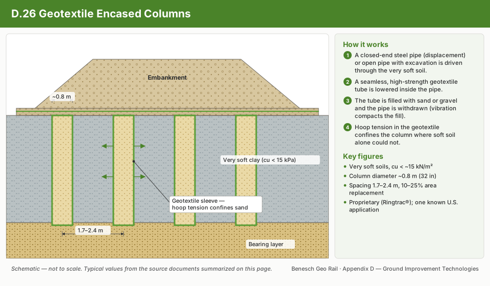
Measured dynamic force of a 20.6-ton padfoot and a 19-ton smooth drum roller on three trial embankments.
Figure 17-LK1. Measured dynamic force of a 20.6-ton padfoot and a 19-ton smooth drum roller on three trial embankments. Source: Look (2023), Figure 7.10-3, p. 235.
Induced compaction (mm) with each pass on the interbedded trial; rebound appears at about 5–6 passes.
Figure 17-LK2. Induced compaction (mm) with each pass on the interbedded trial; rebound appears at about 5–6 passes. Source: Look (2023), Figure 7.10-5, p. 237.

Source: Look, B. G. (2023). Earthworks: Theory to Practice – Design and Construction. CRC Press/Balkema. Case study §7.10, pp. 232–236. Summarized and paraphrased; figures reproduced for internal reference. Full reference under Supplemental Sources.

Case Study 17.17.2 — Wick-drain rigs on dredged sand over 104 psf clay: four ways to size the platform
Case study · Look (2023) §12.7

Related section: 17.3 Prefabricated Vertical Drains (PVDs) with Staged Loading

At the Port of Brisbane reclamation, wick-drain rigs had to work for nine months on 31 acres of dredged sand, about 8.2 ft thick, over Holocene clay with a design undrained strength of 104 psf in the top 20 ft (Look and Honeyfield, 2016). Mud waves during filling left the sand thickness uncertain. BR470 is outside its range here, both for clay under 420 psf and for platform thickness to load width (D/W) above 1.5; it was used for the preliminary design for want of anything better.

Loads. The heaviest rig did not exert the highest pressure: the 50-ton CAT on narrower tracks produced 3,500 psf against 2,030 psf for the 89-ton machine. Check every rig.

Parameters. 27 LFWD tests, 8 DCPs and 4 borehole shear tests gave the sand properties. Two proof-roll passes raised the LFWD modulus by about 20% and reduced its scatter (10th percentile 4,400 psi rolled against 3,260 psi unrolled). Groundwater was found at 6.2–10 ft, not the 20 in. assumed. Clay directly under the sand measured 42–380 psf.

Four answers.

  • BR470 deterministic: 7.5 ft required.
  • BR470 with a PERT distribution and Latin Hypercube simulation: baseline 7 ft; 7.5 ft has under 5% probability of being exceeded. Subgrade strength dominates the tornado chart.
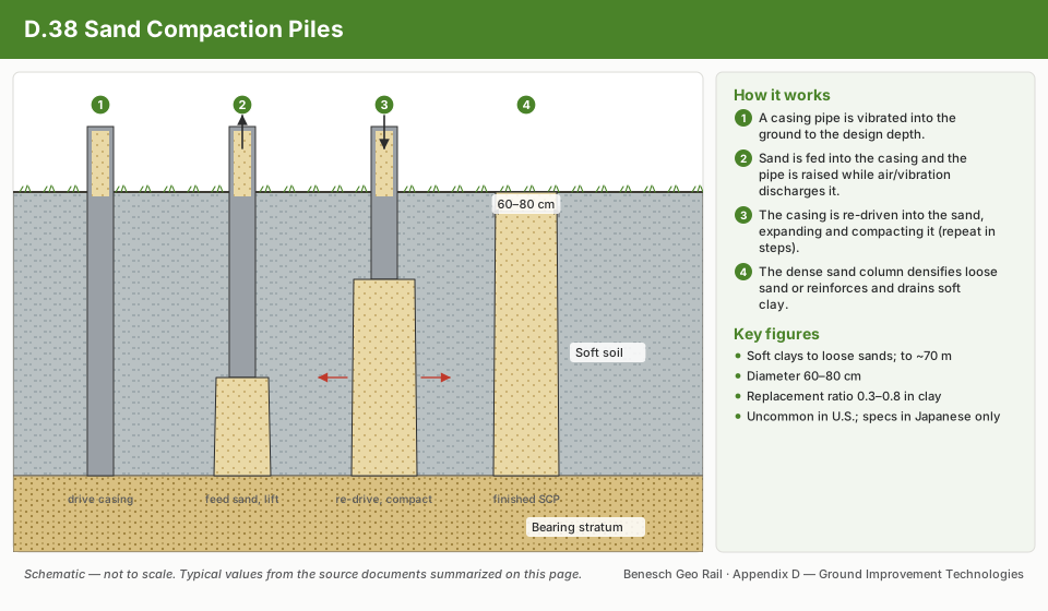
  • Finite element displacement, calibrated to proof-roll ruts, with a 3 in limit: 6.9 ft.
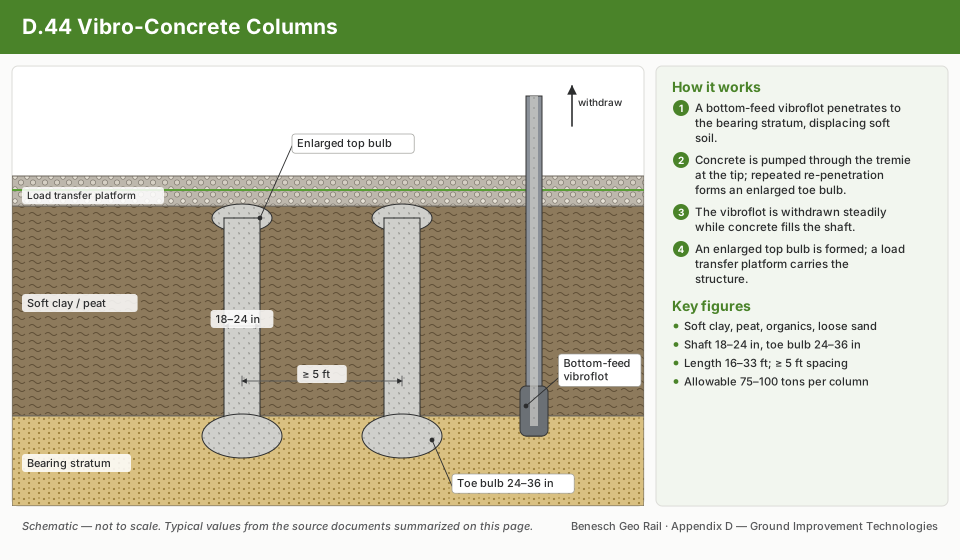
  • Finite element stress at the sand/clay interface against a lower-bound bearing factor Nc = 3.14 for combined shear, as mud waves imply: 7 ft.

Proof rolling as the check. A loaded proof truck will bog rather than topple, while an eccentrically loaded rig can topple, so the truck is the safer test. Proof rolling only means something with a defined vehicle and an acceptance deflection. A rock-filled truck loaded more evenly than a water truck (whose load sloshes) and was preferred. Mean ruts were 3.7 in. after one pass and 5.2 in. after two, and 4.7 in was adopted as the acceptance criterion.

Table 17-LK2. Wick-drain rigs and track pressures (after Look 2023, Table 12.20)

RigWeight (tons)Track width (ft)Critical track pressure
Komatsu excavator6532,700 psf
CAT excavator5033,500 psf
Komatsu excavator894.32,030 psf

For railroad work: ground improvement under new embankments on soft soil, such as wick drains for a yard expansion or a new grade across a marsh, puts the rigs on exactly this kind of platform. Size it by more than one method and calibrate the proof roll before the rigs move on.

Issues considered for the platform: load, rig type, parameters, thickness, groundwater and methodology (Look and Honeyfield 2016).
Figure 17-LK3. Issues considered for the platform: load, rig type, parameters, thickness, groundwater and methodology (Look and Honeyfield 2016). Source: Look (2023), Figure 12.7-1, p. 437.
Measuring proof-roll rut depth; LFWD tests were run in and away from the wheel path (Look and Honeyfield 2016).
Figure 17-LK4. Measuring proof-roll rut depth; LFWD tests were run in and away from the wheel path (Look and Honeyfield 2016). Source: Look (2023), Figure 12.7-8, p. 445.

Source: Look, B. G. (2023). Earthworks: Theory to Practice – Design and Construction. CRC Press/Balkema. Case study §12.7, pp. 432–446. Summarized and paraphrased; figures reproduced for internal reference. Full reference under Supplemental Sources.

Case Study 17.17.3 — Lime-treated local soil in a reinforced slope: choosing by total internalised cost
Case study · Look (2023) §12.8

Related section: 17.7 Lime and Cement Stabilization

Prolonged rain in 2010/11 triggered a 656 ft landslide under a Sunshine Coast hinterland road, in colluvium up to 20 ft thick below a steep escarpment (Look 2012; Chew et al. 2012; Boyer et al. 2013). Five remediation options were compared on total internalised cost: construction cost plus embodied energy, greenhouse-gas emissions from fuel, transport and materials, and the cost of damage to local roads from heavy trucks hauling material. Environmental costs ranged from 2% to 23% of construction cost.

Options 3 and 4 had the lowest totals. Option 3 was chosen because the road authority wanted the fewest heavy trucks on local roads, and lime treatment let the high-plasticity “unsuitable” colluvium be screened of boulders and reused. With 4% hydrated lime cured seven days, shear box cohesion rose from about 420 psf to 1,250–2,200 psf at a similar friction angle; the design still used a softened cohesion of 104 psf.

The work was done in five stages with soil-nailed temporary slopes, drainage slots and regular inclinometer and survey monitoring. When inclinometer 2 showed excessive movement, inspection found a tree at the crown destabilised by the excavation. Once it was felled, the movement stopped.

Table 17-LK3. Remediation options, 2011 AU$ (after Look 2023, Table 12.23, from Chew et al. 2012)

OptionConstructionEnvironmentalTotal internalised
1. Cast-in-place pile wall with ground anchors*3,300,00067,0003,367,000
2. Rockfill buttress3,800,000628,0004,428,000
3. Reinforced fill slope, lime-treated local soil2,400,000278,0002,678,000
4. Reinforced fill slope, imported granular fill2,000,000452,0002,452,000
5. Earth fill embankment with rock toe3,200,000444,0003,644,000
* Greatest technical uncertainty.

For railroad work: slide repairs on remote lines face the same haul-cost and community questions. Reusing treated local soil cuts truck traffic on rural roads, and staged excavation with inclinometers is the standard of care on an active slide.

Cross section through the 660 ft landslide in up to 20 ft of colluvium (Chew et al. 2012).
Figure 17-LK5. Cross section through the 660 ft landslide in up to 20 ft of colluvium (Chew et al. 2012). Source: Look (2023), Figure 12.8-1, p. 447.
Inclinometer 2 showed excessive movement, traced to a crown tree destabilised by the excavation.
Figure 17-LK6. Inclinometer 2 showed excessive movement, traced to a crown tree destabilised by the excavation. Source: Look (2023), Figure 12.9-3, p. 449.

Source: Look, B. G. (2023). Earthworks: Theory to Practice – Design and Construction. CRC Press/Balkema. Case study §12.8, pp. 446–448. Summarized and paraphrased; figures reproduced for internal reference. Full reference under Supplemental Sources.

Case Study 17.17.4 — Working platform at the edge of a creek, designed for slope stability
Case study · Look (2023) §12.6

Related section: 17.8 Geosynthetic Reinforcement

A bridge pier at the edge of a creek, with the next pier 8 ft into it, needed a platform for a BG28 piling rig for a day and an outrigger crane for beam lifting. The temporary-works designer rightly declined to design it with the standard method, since slope stability over soft clay governed. Sheet piling would have cost almost five times the roughly AU$100,000 (2015) platform. Moving the pier a few meters would have removed the problem, which shows why constructability belongs in design.

A deep rock-fill replacement moved the critical slip surface deeper, with high-strength geogrids within the rock fill. Stability was checked separately for standing (uniform 3,800 psf, FS 1.5, above the 1.3 usually accepted for temporary works), penetrating (uniform and trapezoidal, FS 1.3) and extracting. The extracting case was the most critical (FS 1.2) even though its 5,500 psf design pressure is lower than penetration’s 6,400 psf, because of where the load sits. Large plate load tests were run but cannot test a deep slip surface, so an excavator was walked along the edge first. The work went without incident, though rig depressions had to be repaired before the outrigger came on.

Table 17-LK4. Design pressures for the BG28 piling rig (after Look 2023, Table 12.19)

OperationDesign pressureFactor of safety adopted
Handling / transporting / standing3,780 psf1.5
Penetration6,390 psf1.3
Extracting5,470 psf1.2 (critical, trapezoidal)

For railroad work: bridge replacement platforms beside streams and next to embankment slopes need a global stability check for each rig operation, not only a bearing check. The extract phase and the outrigger reactions are often the governing cases.

Platform beside the creek, edge checked with an excavator before the piling rig moved on; design section with multiple high-strength geogrids.
Figure 17-LK7. Platform beside the creek, edge checked with an excavator before the piling rig moved on; design section with multiple high-strength geogrids. Source: Look (2023), Figure 12.6-2, p. 433.

Source: Look, B. G. (2023). Earthworks: Theory to Practice – Design and Construction. CRC Press/Balkema. Case study §12.6, pp. 430–432. Summarized and paraphrased; figures reproduced for internal reference. Full reference under Supplemental Sources.

Author and Sources

Authors: Daniel P. Colwell and Mario Ruel. This chapter was written and compiled by Daniel P. Colwell and Mario Ruel for Railway Ground Hazard Risk Management.
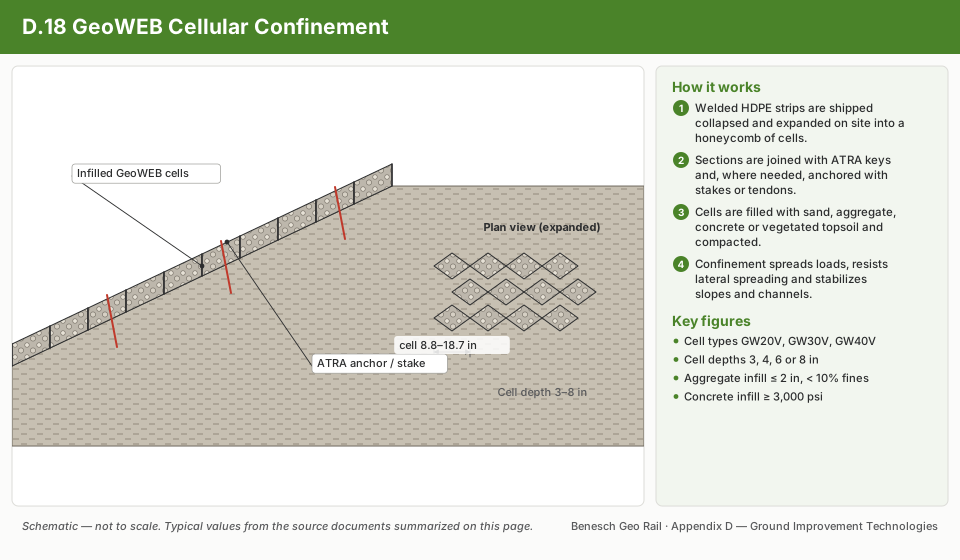
Technical content is drawn from the published sources below, and credit for that material belongs to their authors and publishers. Tables, equations and figures taken from a specific source are also cited where they appear.

Primary sources

  • USACE EM 1110-1-1804, Geotechnical Investigations (2001)
  • FHWA NHI-06-019, Ground Improvement Methods (2006)
  • Barron (1948); Priebe (1995)
  • Kirsch, K. and Bell, A. (2012). Ground Improvement
  • ASTM D698, D1557
  • AREMA MRE Chapter 1

Supplemental sources (LEVI Library)

  • Blacklock, J. R. and Lawson, C. H. (1977). Handbook for Railroad Track Stabilization Using Lime Slurry Pressure Injection. FRA/ORD-77/30, Federal Railroad Administration
  • Pengelly, A. D. Injection for Railroad Subgrades. Hayward Baker, Inc. (scanned; text recovered by OCR)
  • Hayward Baker, Inc. Railroad Subgrade Stabilization (brochure)
  • National Lime Association (2004). Lime-Treated Soil Construction Manual: Lime Stabilization & Lime Modification, Bulletin 326
  • SHRP2 R02 / GeoTechTools (2012). Column-Supported Embankments — fact sheet, design guidance and photographs
  • SHRP2 R02 / GeoTechTools (2012). Rapid Impact Compaction and Jet Grouting fact sheets
  • Schaefer, V. R. et al. (2017). Ground Modification Methods Reference Manual, Vol. I. Geotechnical Engineering Circular No. 13, FHWA-NHI-16-027
  • Look, B. G. (2023). Earthworks: Theory to Practice – Design and Construction. CRC Press/Balkema. Case studies §7.10, §12.6, §12.7, §12.8

File locations for these documents are listed under Supplemental Sources — LEVI Library.

Project management sources

  • Sears, S. K., Sears, G. A., Clough, R. H., Rounds, J. L., and Segner, R. O., Jr. (2015). Construction Project Management: A Practical Guide to Field Construction Management, 6th ed. Hoboken, NJ: John Wiley & Sons
  • Bull, J. W. (ed.) (2015). Life Cycle Costing for the Analysis, Management and Maintenance of Civil Engineering Infrastructure. Dunbeath, Scotland: Whittles Publishing
  • Miller, D. P. (2009). Building a Project Work Breakdown Structure: Visualizing Objectives, Deliverables, Activities, and Schedules. ESI International Project Management Series. Boca Raton, FL: Auerbach Publications (CRC Press, Taylor & Francis Group)
  • Kelly, J., Male, S. and Graham, D. (2004). Value Management of Construction Projects. Oxford: Blackwell Science
  • ASCE Construction Institute Committee on Specifications (L. Eckersley, Chair) (2013). Preparation of Construction Specifications for Civil Projects. Reston, VA: American Society of Civil Engineers
  • Sullivan, W. G., Wicks, E. M. and Koelling, C. P. (2015). Engineering Economy, 16th ed. Upper Saddle River, NJ: Pearson
  • Levy, S. M. (2007). Project Management in Construction, 5th ed. New York: McGraw-Hill
Supplemental Sources — LEVI Library

Material in the green “Supplemental reference” boxes throughout this chapter was added from the following documents in the LEVI geotechnical library. Text is summarized or paraphrased; tables are reproduced with their original source noted; figures are reproduced from the cited document for internal reference use. Consult the original document before relying on a value for design. Blocks marked “After UFC 4-860-01FA (2004)” draw on item S10 and are rewritten for railroad clients. Blocks marked “After Selig & Waters (1994)” summarize item S11 for railroad clients; tables are condensed from the book and its figures are not reproduced. The Case Studies section summarizes case studies from item S12 by Burt G. Look; its figures are reproduced from the book for internal reference use, and the closing “For railroad work” note in each case study is added by the authors of this manual. Blocks tagged “Project management” summarize methods, examples and figures from the project-management, estimating and construction-management books listed here, applied to railroad work; the closing “For railroad work” note in each block is added by the authors of this manual.

  1. Blacklock, J. R. and Lawson, C. H. (1977). Handbook for Railroad Track Stabilization Using Lime Slurry Pressure Injection. FRA/ORD-77/30, Federal Railroad Administration
  2. Pengelly, A. D. Injection for Railroad Subgrades. Hayward Baker, Inc. (scanned; text recovered by OCR)
  3. Hayward Baker, Inc. Railroad Subgrade Stabilization (brochure)
  4. National Lime Association (2004). Lime-Treated Soil Construction Manual: Lime Stabilization & Lime Modification, Bulletin 326
  5. SHRP2 R02 / GeoTechTools (2012). Column-Supported Embankments — fact sheet, design guidance and photographs
  6. SHRP2 R02 / GeoTechTools (2012). Rapid Impact Compaction and Jet Grouting fact sheets
  7. Schaefer, V. R. et al. (2017). Ground Modification Methods Reference Manual, Vol. I. Geotechnical Engineering Circular No. 13, FHWA-NHI-16-027
  8. Profillidis, V. A. (2014). Railway Management and Engineering, 4th ed. Farnham, UK: Ashgate. Chapters 7–9, 11–13, 16–17, 20 and 22 (track system, mechanical behavior of track, subgrade, sleepers, ballast, transverse effects, maintenance, slab track, electrification foundations, safety)
  9. Benesch. Geotechnology for Railroaders Program, Modules 1–8 (two-day training course reference: risk management, geology and soils, ballast and sub ballast, drainage, slides, slope and subgrade stabilization, scour, rock falls, beaver dams, winter problems, spring thaw, extreme weather, earthquakes). Field photographs and figures from the course; slope stabilization process slides adapted from material by D. Colwell
  10. U.S. Army Corps of Engineers, Naval Facilities Engineering Command and Air Force Civil Engineer Support Agency (2004). UFC 4-860-01FA, Railroad Design and Rehabilitation. Unified Facilities Criteria, 16 January 2004 (supersedes TI 850-02, 1 March 2000); approved for public release, distribution unlimited. Used on this page: ch. 6 (§8) and ch. 9 (§4)
  11. Selig, E. T. and Waters, J. M. (1994). Track Geotechnology and Substructure Management. London: Thomas Telford. Used on this page: chs. 11 and 12
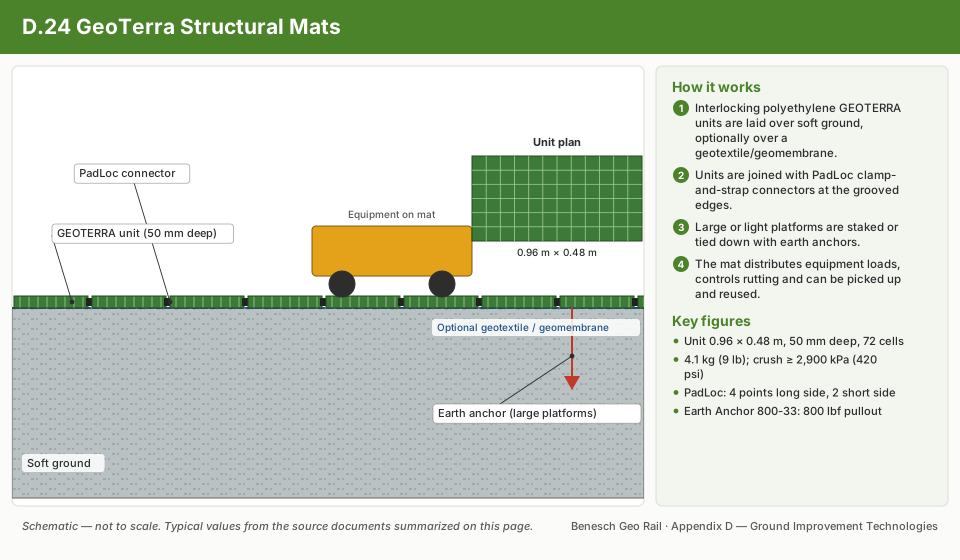
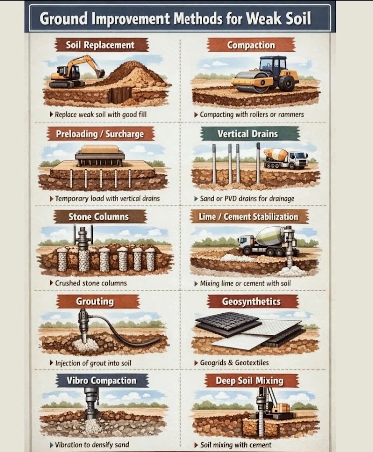
  12. Look, B. G. (2023). Earthworks: Theory to Practice – Design and Construction. Leiden: CRC Press/Balkema (Taylor & Francis). ISBN 978-1-032-10470-6. Case studies used on this page: §7.10, §12.6, §12.7, §12.8
  13. Sears, S. K., Sears, G. A., Clough, R. H., Rounds, J. L., and Segner, R. O., Jr. (2015). Construction Project Management: A Practical Guide to Field Construction Management, 6th ed. Hoboken, NJ: John Wiley & Sons. Used on this page for project-management material
  14. Bull, J. W. (ed.) (2015). Life Cycle Costing for the Analysis, Management and Maintenance of Civil Engineering Infrastructure. Dunbeath, Scotland: Whittles Publishing. Used on this page for project-management material
  15. Miller, D. P. (2009). Building a Project Work Breakdown Structure: Visualizing Objectives, Deliverables, Activities, and Schedules. ESI International Project Management Series. Boca Raton, FL: Auerbach Publications (CRC Press, Taylor & Francis Group). Used on this page for project-management material
  16. Kelly, J., Male, S. and Graham, D. (2004). Value Management of Construction Projects. Oxford: Blackwell Science. Used on this page for project-management material
  17. ASCE Construction Institute Committee on Specifications (L. Eckersley, Chair) (2013). Preparation of Construction Specifications for Civil Projects. Reston, VA: American Society of Civil Engineers. Used on this page for project-management material
  18. Sullivan, W. G., Wicks, E. M. and Koelling, C. P. (2015). Engineering Economy, 16th ed. Upper Saddle River, NJ: Pearson. Used on this page for project-management material
  19. Levy, S. M. (2007). Project Management in Construction, 5th ed. New York: McGraw-Hill. Used on this page for project-management material
← Previous · Part VII Chapter 16 — Retaining Structures
Next · Part VIII → Chapter 18 — Pavement Subgrade Evaluation