
Geotechnical engineering libraryContact
Railroad Geotechnical Services Manual | Primary Source: USACE EM 1110-1-1804 All equations and parameters expressed in English (Imperial) units throughout.
Apps on dirtbert.com that support this chapter. Each one runs in a web browser on a desktop or a phone, with nothing to install. How to use the apps (I.3).
NANCY pages ask you to accept the Use and Disclaimers once in each browser.
Settlement analysis is the serviceability companion to the bearing capacity calculations developed in Chapter 11. For railroad infrastructure, settlement governs more designs than bearing capacity failure — particularly embankment fills over soft alluvial soils, approach fills behind bridge abutments, and intermodal yard slabs on compressible clay. Total settlement S_total consists of three components: immediate (elastic) settlement S_i, primary consolidation settlement S_c, and secondary compression S_s. Time-rate analysis using Terzaghi's consolidation theory predicts when settlement will occur, enabling the consultant to recommend preloading, staged construction, or ground improvement to achieve acceptable geometry before track placement. This chapter develops all three settlement components in English units, cross-references FRA track geometry tolerances by track class as the acceptance criteria, and presents worked examples for a CSXT embankment over soft clay, a CN bridge approach fill with time-rate prediction, and a BNSF intermodal yard slab on overconsolidated clay. All nine railroad client standards are integrated throughout.
FRA track geometry tolerances (49 CFR Part 213) establish the operational framework within which all settlement predictions must be evaluated. Unlike building foundations, where total settlement of 1–2 in. is routinely acceptable, railroad track geometry tolerances are measured in fractions of an inch — the structural consequence of derailment, speed restriction, or emergency slow order is immediate and measurable.
| Track Class | Max Speed (Freight) | Cross-Level Tolerance | Surface (Runoff) Tolerance | Total Settlement Limit (our recommendation) | Angular Distortion Limit |
|---|---|---|---|---|---|
| Class 1 | 10 mph | 3.0 in. | 3.0 in. per 62 ft | ≤ 3.0 in. | ≤ 1/200 |
| Class 2 | 25 mph | 2.0 in. | 2.0 in. per 62 ft | ≤ 2.0 in. | ≤ 1/300 |
| Class 3 | 40 mph | 1.75 in. | 1.75 in. per 62 ft | ≤ 1.5 in. | ≤ 1/400 |
| Class 4 | 60 mph | 1.5 in. | 1.5 in. per 62 ft | ≤ 1.0 in. | ≤ 1/500 |
| Class 5 | 80 mph | 0.75 in. | 0.75 in. per 62 ft | ≤ 0.75 in. | ≤ 1/700 |
| Class 6 | 110 mph | 0.5 in. | 0.5 in. per 62 ft | ≤ 0.5 in. | ≤ 1/1,000 |
| Class 7 (Amtrak NEC) | 125 mph | 0.5 in. | 0.5 in. per 62 ft | ≤ 0.375 in. | ≤ 1/1,500 |
Angular distortion δ/L (where δ = differential settlement between two points, L = distance between them) is the critical parameter for bridge approach transitions and structure-embankment interfaces. Amtrak ES and NSR ESM independently impose tighter limits than FRA at structure transitions.
Railroad client settlement requirements beyond FRA minima:
Elastoplastic finite-element results reproduced by Profillidis show the settlement under a passing axle at the top of subgrade, at the tie and at the rail for subgrade classes S1, S2, S3 and rock, for track-bed thicknesses of 12–39 in.. Subgrade class dominates: moving from S1 to S3 cuts the settlement several-fold, while extra track-bed thickness gives a smaller, steady reduction. Tie type matters less than subgrade class.
For new fills, the book reminds designers to overbuild embankment width and height to allow for the fill’s own compaction after construction (Chapter 3, §3.2).
Figures · click to zoom
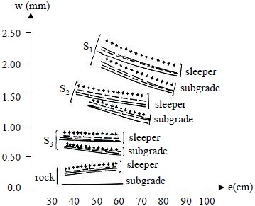
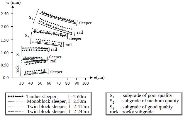
After Profillidis (2014), §8.4.7, Figs. 8.8–8.9. Full reference under Supplemental Sources.
Before computing settlement, the change in vertical stress Δσ_v at depth z due to the applied load must be determined. For a uniformly loaded rectangular area of width B and length L at the surface:
Δσ_v = q · I_σ
Where I_σ is the Boussinesq influence factor (Newmark, 1935), a function of m = B/z and n = L/z:
I_σ = (1/4π)[2mn√(m²+n²+1)/(m²+n²+1+m²n²) × (m²+n²+2)/(m²+n²+1)
+ arcsin(2mn√(m²+n²+1)/(m²+n²+1+m²n²))]
For practical use, Boussinesq influence charts (or tables) are used; I_σ ranges from 0.25 (square footing, z = 0) to near zero at large depth. For a 2:1 stress distribution approximation (AREMA MRE Chapter 8 simplification), commonly used for preliminary analysis:
Δσ_v = Q / [(B + z)(L + z)] (psf)
Where Q = total load (lb), B and L = footing dimensions (ft), z = depth below footing base (ft). For strip loads (railroad embankments):
Δσ_v = (q/π)[β + sin β · cos(β + 2δ)] (psf)
Where β = the angle subtended by the load width at depth z (radians), δ = angle from load centerline, q = applied surface pressure (psf). For the centerline of a strip load:
Δσ_v,center = (q/π)[β + sin β]
Immediate settlement occurs under undrained loading conditions in saturated cohesive soils, or drained loading in granular soils. It develops essentially instantaneously upon load application.
Si = q · B · (1 − μ²) / Es · Iw
Where:
| Soil Type (USCS) | E_s (psf) | Typical Source |
|---|---|---|
| Very soft clay (CH) | 10,000–25,000 | Unconfined compression |
| Soft clay (CL) | 25,000–75,000 | Unconfined compression |
| Medium stiff clay | 75,000–150,000 | CPTu, PMT |
| Stiff clay | 150,000–300,000 | CPTu, PMT |
| Very stiff clay | 300,000–500,000 | PMT, pressuremeter |
| Loose sand (SP/SM) | 100,000–250,000 | SPT correlation |
| Medium-dense sand | 250,000–500,000 | SPT correlation |
| Dense sand/gravel | 500,000–1,500,000 | SPT correlation |
Immediate settlement is critical for UPRR intermodal yard slab design and for any structure where the total settlement is dominated by granular or stiff-clay subgrades. For most railroad embankment designs over soft cohesive soils, primary consolidation governs and S_i is secondary.
Eq. 12-4 assumes a single modulus for the whole stressed zone. For footings, signal foundations and yard slabs on sand, USACE EM 1110-1-1904 recommends Schmertmann’s approximation, which sums strain over sublayers of thickness Δz = 0.2B using a triangular strain-influence diagram (Figure 12-S1):
ρi = C1 · Ct · Δp · Σ (Izi / Esi) Δzi
Because the method weights the stiffness of each sublayer, it captures a loose sand seam at depth B/2 that a single-modulus calculation averages away.
Source: U.S. Army Corps of Engineers (1990). Settlement Analysis. EM 1110-1-1904
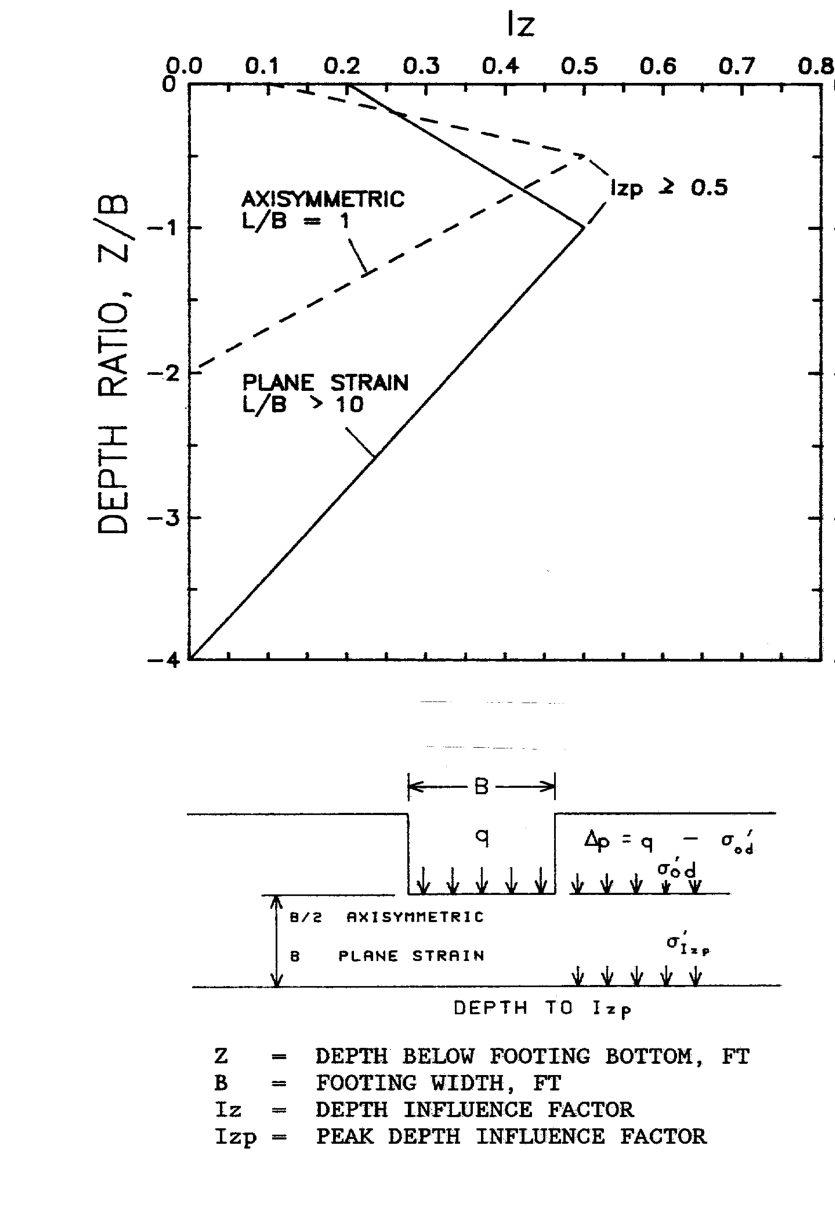
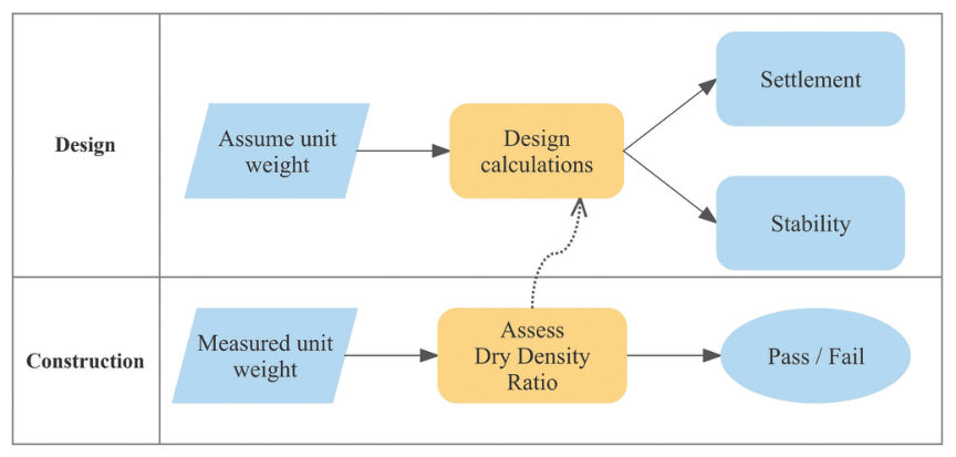
Case study: 12.16.1 Unit weight of fill: design assumes 127 pcf, the job measures more (Look 2023), in §12.16 Case Studies.
Primary consolidation settlement S_c is governed by the compressibility of the clay skeleton as excess pore pressures dissipate. Three cases apply depending on the preconsolidation stress σ'_p:
Reference graphics · click to zoom
Sc = [Cc / (1 + e₀)] · H · log[(σ'_v0 + Δσ) / σ'_v0]
Sc = [Cs / (1 + e₀)] · H · log[(σ'_v0 + Δσ) / σ'_v0]
Sc = [Cs / (1 + e₀)] · H · log[σ'_p / σ'_v0]
+ [Cc / (1 + e₀)] · H · log[(σ'_v0 + Δσ) / σ'_p]
Where:
Cc = 0.009 · (LL − 10)
Where LL = liquid limit (%). Valid for normally consolidated clays; use with caution for organic soils. For railroad projects, laboratory consolidation tests (ASTM D 2435) are required by CSXT ES, NSR ESM, BNSF EI, and Amtrak ES for all embankments exceeding 6 ft over soft clay.
e₀ = (Gs · γ_w / γ_d) − 1
Where G_s = specific gravity (≈ 2.70 for most clays), γ_d = dry unit weight (pcf), γ_w = 62.4 pcf.
When a compressible layer is thick (> 5 ft) or when the stress increase varies significantly with depth, the layer should be divided into sublayers of 2–4 ft thickness. Settlement is computed for each sublayer at its midpoint stress state, then summed:
Sc,total = Σ [Cc,i / (1 + e₀,i)] · Hi · log[(σ'_v0,i + Δσ_i) / σ'_v0,i]
This sublayer approach is mandatory for BNSF and Amtrak projects with clay layers > 10 ft thick, where ignoring stress variation underestimates settlement at the top of the layer and overestimates at depth.
Organic soils can compress by up to about 40% (12 ft of peat can mean 5 ft of settlement). Muskeg also punches under load, and buried corduroy decays. At Bedford Mile 29.8, years of swamp ties never stopped the settlement; only a proper berm, together with draining the water driving the movement, solved it. At Lac la Biche Sub Mile 173.48, 400 ft of differential settlement into deep peat needed piles. In 2016 dollars, swamp ties cost about $670,000 per mile, against about $280,000 per mile for undercutting and about $6.7 million per mile for new track (course figures of $600,000, $250,000 and $6,000,000 in 2012 dollars, escalated by the ENR Construction Cost Index; see Chapter 17, Table 17-6), so diagnosing the mechanism early is the cheapest option.
Figures · click to zoom
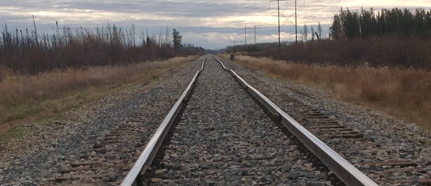
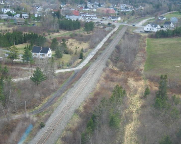
After Geotechnology for Railroaders Program, Module 2, Module 6.1, Module 6.2; Module 2 §08; Module 6.1 §03; Module 6.2 §01, §05. Full reference under Supplemental Sources.
The degree of consolidation U (fraction of ultimate settlement completed at time t) is governed by the dimensionless time factor T_v:
Reference graphics
Reference graphics · click to zoom
Tv = cv · t / H_dr²
Where:
| U (%) | T_v (simplified) | T_v (exact) |
|---|---|---|
| 10 | 0.008 | 0.008 |
| 20 | 0.031 | 0.031 |
| 30 | 0.071 | 0.071 |
| 40 | 0.126 | 0.126 |
| 50 | 0.197 | 0.197 |
| 60 | 0.287 | 0.287 |
| 70 | 0.403 | 0.403 |
| 80 | 0.567 | 0.567 |
| 90 | 0.848 | 0.848 |
| 95 | 1.163 | 1.129 |
| 99 | — | 1.781 |
For U ≤ 60%:
Tv = π/4 · (U/100)² (simplified parabolic approximation)
For U > 60%:
Tv = −0.933 · log(1 − U/100) − 0.085
S(t) = U · Sc,total
t = Tv · H_dr² / cv
| Soil Type | c_v (ft²/day) | c_v (ft²/year) | Notes |
|---|---|---|---|
| Soft organic clay | 0.0005–0.005 | 0.2–2 | CSXT coastal Georgia, CN Manitoba |
| Soft marine clay | 0.005–0.05 | 2–18 | NSR tidewater VA, Amtrak NEC |
| Medium clay | 0.05–0.2 | 18–73 | BNSF Kansas, UPRR Nebraska |
| Stiff clay | 0.2–1.0 | 73–365 | NSR Appalachian residual |
| Very stiff clay | 1.0–10 | 365–3,650 | Quick-draining; settle rapidly |
| Silty clay (CL-ML) | 0.1–0.5 | 37–183 | CPKC Prairie provinces |
Multiplying path length squared by unit conversion: if c_v in ft²/day and H_dr in ft, time t is in days.
Secondary compression occurs after primary consolidation is essentially complete (U ≈ 95–100%) as the clay skeleton continues to creep under sustained load. It is particularly significant for organic soils (Pt) and highly plastic clays (CH) — common in CSXT Georgia coastal swamps, CN Manitoba peatlands, and BNSF Louisiana territory.
Ss = Cα / (1 + ep) · H · log(t₂ / t₁)
Where:
Cα/Cc ≈ 0.04 ± 0.01 (for inorganic clays)
Cα/Cc ≈ 0.05 to 0.07 (for organic clays and peats)
For a 50-year railroad service life (t₂ = 18,250 days) with primary consolidation completing at t₁ = 500 days, log(18,250/500) = log(36.5) = 1.562. Even a modest C_α = 0.010 over a 10 ft clay layer produces S_s = 0.010/(1 + 1.8) × 10 × 1.562 = 0.056 ft = 0.67 in — significant on a Class 5 mainline with a 0.75 in. tolerance.
USACE EM 1110-1-1904 (Table 3-14, after Mesri) extends the ratios in Eq. 12-15 to other materials encountered on railroad alignments:
Table 12-S1. Ratio of secondary compression index to compression index
| Soil | Cα/Cc |
|---|---|
| Inorganic soils | 0.025–0.060 |
| Clay | 0.025–0.085 |
| Silt | 0.030–0.075 |
| Peat | 0.030–0.085 |
| Muskeg | 0.090–0.100 |
For a first approximation before tests are available, USACE (after NAVFAC DM-7.1) gives Cα ≈ 0.0001 wn for natural water contents 10–3,000%. The manual cautions that sample disturbance lowers the measured Cα in the virgin range and that secondary-compression predictions “have often not been reliable” — one more reason to confirm long-term behavior with settlement plates rather than rely on the calculation alone.
Source: U.S. Army Corps of Engineers (1990). Settlement Analysis. EM 1110-1-1904
Lea and Brawner’s British Columbia highway experience gives practical guidance for the peat and muskeg crossings noted above:
Source: Lea, N. D. and Brawner, C. O. Highway Design and Construction Over Peat Deposits in Lower British Columbia. Highway Research Board
S_total = Si + Sc + Ss
α = (S_A − S_B) / L_AB
Where S_A and S_B are predicted settlements at two adjacent structures or reference points, and L_AB is the distance between them (ft). AREMA MRE Chapter 8 limits angular distortion at bridge approach transitions to 1/500 for Class 4 track.
Bridge Approach Transition: The most critical angular distortion check in railroad geotechnical practice is at the abutment–embankment interface. A rigid pile-supported abutment settling < 0.1 in. adjacent to an approach fill settling 3.0 in. over 30 ft produces α = 2.9/30 = 0.097 — far exceeding any FRA class limit. AREMA Chapter 8, CSXT ES, and NSR ESM all require approach slab design or engineered approach fill to limit this transition zone differential.
Repeated and dynamic loads. USACE EM 1110-1-1904 notes that loose sands compact under vibration and that this is a major cause of differential settlement. Cohesionless soils with Dr above about 75% should not settle significantly, although intense dynamic loading can still compact dense sand by 1–2% of the stratum thickness. Dynamic settlement may be insignificant if the combined static and dynamic bearing stress stays below one-half of the allowable bearing capacity. Errors in dynamic-settlement predictions can be 50% or more. For clays under repeated deviator stress (0.1–10 Hz, a typical range for traffic), the manual gives a creep-strain-rate formulation from cyclic triaxial tests but warns it may underestimate settlement because traffic loading is more complex than repeated vertical load.
Collapsible soils. Loess, some alluvial fans and cemented silts lose their bonded structure on wetting. Typical collapsible soils are light-colored, LL < 45, PI < 25, with dry unit weight 65–105 pcf; collapse rarely occurs below 40% porosity. USACE notes that dynamic loading can also break the bonds, “particularly important for roads, airfields, railways.”
Table 12-S2. Wetting that can trigger collapse (EM 1110-1-1904, Table 5-4, condensed)
| Type of wetting | Railroad example | Result |
|---|---|---|
| Local, shallow | Blocked ditch, leaking pipeline crossing | Settlement in the upper layer within the wetted area |
| Intense local | Industry effluent, broken water main, irrigation | Can saturate the whole collapsible zone in < 1 year; uneven, damaging settlement |
| Slow, uniform groundwater rise | Reservoir or regional water table rise | Uniform, gradual settlement |
| Slow increase in water content | Reduced evaporation under a paved yard or slab | Incomplete, progressive settlement |
Collapse potential CP (Jennings and Knight, 1975) is the strain on flooding a consolidometer specimen at 2 tsf: 0–1% negligible, 1–5% moderate trouble, 5–10% trouble, 10–20% severe trouble, > 20% very severe trouble. For design, load the specimen to the anticipated field stress and then inundate it (ASTM D4546, Method B); settlement = [(eo − ec)/(1 + eo)]H. USACE cautions that lab tests can miss soil that later collapses in the field, and the amount depends on how far the wetting front travels — so drainage control is part of the design.
Source: U.S. Army Corps of Engineers (1990). Settlement Analysis. EM 1110-1-1904
Geometry limits put a practical ceiling on differential settlement under track. European intervention limits for the longitudinal (surface) defect on a 33-ft chord range from about 0.35–0.47 in. at 87–99 mph to 0.55–0.83 in. below 37 mph (Chapter 3, §3.11). Emergency speed restrictions begin at 0.71 in.. Because the chord is short, these are effectively limits on settlement differences over about 33 ft. Embankment, culvert and transition settlement predictions should be checked against that scale, not only against total settlement.
After any surfacing, defects grow quickly up to about 2 million tons of traffic and then slowly, roughly with log T, at a rate (0.079–0.24 in. per decade of traffic) that depends mainly on subgrade quality (Chapter 4, §4.10).
Figures · click to zoom
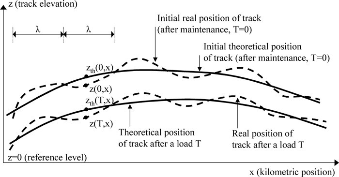
After Profillidis (2014), §16.3, §16.6–16.7, Fig. 16.2. Full reference under Supplemental Sources.
Components. Total settlement is the sum of three parts:
On new track, more than half comes from the ballast. After each tamping the ballast share grows again, because the loosened top ballast starts over.
Use a power law, not a semilog fit. Settlement after N load cycles fits SN = S1 Nb, with b typically 0.10–0.18. A semilog fit increasingly underpredicts at large N, and so overestimates the time to the next surfacing.
Load cycles per MGT. Cm = 106 ÷ (Aa × Na), where Aa is axle load in tons and Na is axles per load cycle. Use Na = 2 per car for ballast. For example, a 39-ton axle gives about 12,800 cycles per MGT.
| Layer | Relation | At 100 MGT |
|---|---|---|
| Top 12 in. of ballast (strain) | ε = 0.026 T0.21 | ε ≈ 0.068 → 0.8 in. |
| Subballast (strain) | ε = 0.017 T0.16; about 2.6 × 10⁻⁵ per MGT beyond ~150 MGT | ε ≈ 0.036 |
| Subgrade, top 10 ft of moist fine silty sand | S (in.) = 0.039 T0.37 (typical); 0.054 T0.52 (worst section) | ≈ 0.2 in. (typical) |
| Subgrade, long term | 0.001–0.0026 in. per MGT, linear beyond ~50 MGT | — |
the authors evaluated the 100 MGT column from the relations. Rapid compression occurred through the first ~3 MGT, then continued at a slower rate.
Lift and settlement. After a low lift, the track settles back by about the amount it was lifted within roughly a year, so the change does not last. Lifts above about 1 in., which exceed the ballast D50, leave a residual lift. Allow about 0.16 in. of settlement even at zero lift, from wear and compaction.
After Selig & Waters (1994), chs. 8 and 15. Full reference under Supplemental Sources.
When predicted settlement S_c exceeds the client's allowable limit, preloading with temporary surcharge fill is the most cost-effective mitigation. The concept: apply a surcharge load greater than the permanent design load, allow consolidation to occur before track placement, then remove the surcharge and install track on a pre-compressed subgrade.
Reference graphics
Δσ_surcharge = Δσ_permanent × [Sc,required / Sc,total]^(1/(Cc/Cs))
A simplified approach: select q_surcharge such that primary consolidation under q_surcharge equals the sum of primary consolidation + secondary compression expected under q_permanent over the service life. NSR ESM requires this calculation for all bridge approach fills where predicted settlement exceeds 2 in.
t_surcharge = 0.848 · H_dr² / cv
If t_surcharge is prohibitively long (> 6–12 months on a construction schedule), prefabricated vertical drains (PVDs) are combined with the surcharge to accelerate drainage — addressed in Chapter 17 (Ground Improvement).
Lea and Brawner’s case histories from the Vancouver area test the assumptions behind Eq. 12-18 and 12-19:
Source: Lea, N. D. and Brawner, C. O. Highway Design and Construction Over Peat Deposits in Lower British Columbia. Highway Research Board
When surcharge time is not available, or added fill would cause a stability failure, the alternative is to reduce Δσ itself. Three generations of lightweight fill appear in the library:
Table 12-S3. Lightweight fill options
| Material | Key properties | Design notes |
|---|---|---|
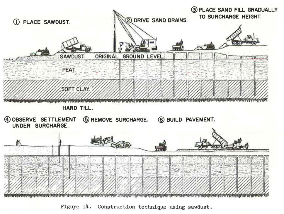
| Sawdust (historic; Trans-Canada Highway, Burnaby) | 3–12 ft thick; compressed to 80–90% of placed thickness under about ½ tsf preload; lab φ = 50° | Rots and can spontaneously combust above the water table, so the top must end up below groundwater after settlement. Settlement had to be predicted accurately to place it at the right grade. |
| Expanded shale, clay or slate (ESCS) lightweight aggregate | Kiln-expanded at 1,900–2,200°F; relative density 1.3–1.6 vs. 2.6–3.0 for normal aggregate (about half the mass per volume); AASHTO M 195 gradations | Open-graded; still needs compaction (lifts ≤ 12 in. loose with vibratory roller). Density control by a one-point Proctor (modified ASTM D698) plus a method spec. |
| EPS geofoam (ASTM D6817) | EPS 15 / 19 / 22 / 29: minimum density 0.90 / 1.15 / 1.35 / 1.80 pcf; compressive resistance at 10% strain 10.2 / 16.0 / 19.6 / 29.0 psi | “Zero net load”: excavate native soil equal in weight to the geofoam plus everything placed on it. It can also replace the active wedge behind an abutment. |
Case: US 17 / SC 707, Myrtle Beach, SC. At the nearby Fantasy Harbour project, embankments 10–42 ft high had settled 9 to 67 in. For the US 17 / SC 707 interchange, bridge approach fills over 30–60 ft of soft to firm clay and loose, liquefiable sands were estimated to settle 78 in. at the abutment if built with normal-weight fill (120 pcf). The design combined LWA borrow to cut the magnitude, PVDs with granular surcharge to speed it, and deep soil mixing for seismic slope stability and abutment performance.
Railroad cautions (engineering judgment, not from the sources): lightweight fills must be covered by enough ballast, subballast and soil to spread axle loads and resist buoyancy at flood stage. Geofoam must be protected from petroleum spills (hydrocarbon-resistant membrane) near fueling or derailment-prone areas. Confirm dynamic stiffness under E-80 loading before using any lightweight fill directly under track.
Source: Lea, N. D. and Brawner, C. O. Highway Design and Construction Over Peat Deposits in Lower British Columbia. Highway Research Board · Speck, J. and Wall, J. Use of Lightweight Aggregate Fill in Highway Projects for Settlement Control and Construction Speed (presentation). Big River Industries / Carolina Stalite Co. · Insulfoam. Geofoam — A Lightweight Fill Alternative (presentation)
Levy (2010) explains, from the owner’s side, how changes interact with the contractor’s critical path method (CPM) schedule. The critical path moves as the job proceeds, and a delay to one critical task can cascade into later tasks and push out the completion date. When a change may affect time, owners face the question of whether the delay is real. Levy advises settling time when the change is priced, not later, because once unrelated contractor delays accumulate it becomes hard to separate them from the change. Extended time matters because general conditions costs (supervision, trailers, utilities, rentals) continue, and he cites $20,000 to $40,000 per month as a typical range.
Where time cannot be agreed, he suggests two approaches: issue the change with a statement that the work proceeds while the owner reserves the right to challenge any time extension, or sign the cost proposal provisionally, reserving the right to challenge both cost and time. Change-order forms often require checking whether the change increases, decreases or does not affect the contract end date, and owners should read that box before signing.
On float, Levy notes that schedules carry a cushion of extra days for weather, late equipment or short crews. Unless the contract says otherwise, that float belongs to the contractor. If the owner wants float for its own contingencies, such as late delivery of owner-furnished items, it must reserve it in the contract; otherwise an owner-caused delay that consumes the contractor’s float can become a claim.
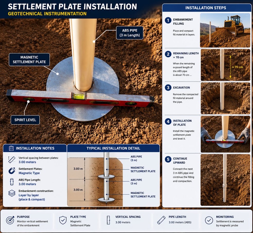
For railroad work: Preload and surcharge programs for embankment widening or approach fills put a waiting period directly on the critical path, and its true length depends on measured consolidation rather than on the design estimate. Specify in the contract who owns float in the hold period, how the hold may be extended or shortened on the basis of settlement plate and piezometer data, and how extended time will be paid. Write the decision rule (for example, release when the monitored settlement rate falls below a stated value) into the special provisions so that a longer hold is a defined outcome rather than a dispute.
Source: Levy, S. M. (2010). Construction Process Planning and Management: An Owner’s Guide to Successful Projects. Burlington, MA: Butterworth-Heinemann (Elsevier), pp. 215–216. Summarized and paraphrased. Full reference under Supplemental Sources.
| Boring | Sample | Depth (ft) | USCS | LL (%) | PI | e₀ | C_c | C_s | C_α | c_v (ft²/day) | OCR | σ'_p (psf) |
|---|---|---|---|---|---|---|---|---|---|---|---|---|
| B-01 | S-3 | 8–10 | CH | 72 | 45 | 1.82 | 0.56 | 0.07 | 0.022 | 0.0032 | 1.0 | 820 |
| B-01 | S-5 | 14–16 | CH | 68 | 41 | 1.71 | 0.52 | 0.065 | 0.021 | 0.0051 | 1.1 | 1,080 |
| B-02 | S-3 | 8–10 | OH | 105 | 63 | 2.45 | 0.88 | 0.11 | 0.062 | 0.0018 | 1.0 | 750 |
| B-02 | S-5 | 14–16 | CH | 74 | 47 | 1.88 | 0.59 | 0.074 | 0.024 | 0.0028 | 1.0 | 1,040 |
| B-03 | S-4 | 11–13 | CL | 48 | 25 | 1.35 | 0.31 | 0.039 | 0.012 | 0.0120 | 1.4 | 1,750 |
| B-03 | S-6 | 18–20 | CH | 69 | 43 | 1.77 | 0.53 | 0.066 | 0.021 | 0.0044 | 1.0 | 1,500 |
Design values selected: C_c = 0.56 (average CH); C_s = 0.07; C_α = 0.022; c_v = 0.004 ft²/day; e₀ = 1.82; one-way drainage (rock at 22 ft depth); H_dr = 14 ft (clay layer 0–22 ft; drainage to surface sand only).
Reference graphics
Project context: CSXT new siding construction, Coastal Georgia. Proposed embankment: 10 ft of structural fill (γfill = 120 pcf) over 14 ft of normally consolidated soft CH clay (C_c = 0.56, e₀ = 1.82, c_v = 0.004 ft²/day, Cα = 0.022). Clay is underlain by dense sand (H_dr = 14 ft, one-way drainage to surface). Water table at 2 ft below original ground. CSXT ES requires total settlement ≤ 1.0 in. for Class 4 siding. Compute S_c and S_s; evaluate FRA compliance.
Step 1 — Initial effective stress at clay midpoint (z = 7 ft below original surface)
Surface to WT (2 ft): σ_v = 120_fill? No — original ground. Use γ_native = 110 pcf above WT.
σ_v(0–2 ft) = 2 × 110 = 220 psf
σ_v(2–7 ft) = 5 × (110 − 62.4) = 5 × 47.6 = 238 psf
σ'_v0 = 220 + 238 = 458 psf
Note: The clay top is at z = 0 ft (native ground surface); the midpoint of the 14-ft clay layer is at 7 ft depth below original surface.
At clay midpoint (7 ft into clay, WT at 2 ft):
Overburden above clay top: 220 psf (2 ft native soil above WT)
Weight of 7 ft of saturated clay: 7 × (110 − 62.4) = 7 × 47.6 = 333 psf
σ'_v0 = 220 + 333 = 553 psf
Step 2 — Stress increase from 10 ft embankment (strip load, B = 40 ft at base, for siding)
Using 2:1 distribution to midpoint of clay (z = 7 ft below fill base):
q_fill = γ_fill × H = 120 × 10 = 1,200 psf
Δσ = q_fill × B / (B + z) = 1,200 × 40 / (40 + 7) = 48,000 / 47 = 1,021 psf
(Full 2:1 formula for strip requires length; for continuous embankment L >> B, use Δσ_v,center ≈ q for z << B. Use Δσ = 1,021 psf as conservative estimate at centerline midlayer.)
Step 3 — Primary consolidation settlement (NC clay, Eq. 12-5)
Sc = [Cc / (1 + e₀)] × H × log[(σ'_v0 + Δσ) / σ'_v0]
= [0.56 / (1 + 1.82)] × 14 × log[(553 + 1,021) / 553]
= [0.56 / 2.82] × 14 × log[1,574 / 553]
= 0.1986 × 14 × log(2.846)
= 0.1986 × 14 × 0.4543
= 1.263 ft = 15.2 in.
Step 4 — Time to 90% consolidation (U = 90%, T_v = 0.848)
H_dr = 14 ft (one-way drainage)
t_90 = T_v × H_dr² / cv = 0.848 × (14)² / 0.004
= 0.848 × 196 / 0.004
= 166.2 / 0.004
= 41,544 days = 113.8 years
This is far too long for a construction schedule. PVDs or surcharge preloading must be specified.
Step 5 — Secondary compression (t₁ = end of primary; t₂ = 50 yr service life)
Assuming PVDs accelerate primary consolidation to t₁ = 180 days; service life t₂ = 50 yr = 18,250 days:
Ss = [Cα / (1 + ep)] × H × log(t₂/t₁)
ep ≈ e₀ − ΔeP = 1.82 − Cc × log(Δσ/σ'_v0 + 1) = 1.82 − 0.56 × log(2.846) = 1.82 − 0.254 = 1.566
Ss = [0.022 / (1 + 1.566)] × 14 × log(18,250/180)
= [0.022 / 2.566] × 14 × log(101.4)
= 0.00857 × 14 × 2.006
= 0.241 ft = 2.9 in.
Step 6 — FRA compliance check
Total post-construction settlement (after 90% primary complete with PVDs + 50 years secondary):
S_total = 0.10 × 15.2 + 2.9 = 1.52 + 2.9 = 4.4 in. >> CSXT limit of 1.0 in. for Class 4
Conclusion: Primary consolidation of 15.2 in. is unacceptably large; PVDs alone will not reduce the magnitude, only the time rate. Ground improvement is required — either (a) preloading with surcharge to achieve > 90% primary consolidation before track, combined with secondary compression acceptance, or (b) deep soil mixing or rigid inclusion columns to reduce compressible layer contribution. See Chapter 17. CSXT ES requires BNSF-equivalent settlement plate monitoring during surcharge loading.
Project context: CN Prairie Subdivision, southern Manitoba. Bridge approach fill: 18 ft over 20 ft of soft silty clay (CL-ML: C_c = 0.35, C_s = 0.04, e₀ = 1.25, c_v = 0.08 ft²/day, OCR = 1.0). Two-way drainage (sand above and below clay). Design fill stress increase at midpoint: Δσ = 1,440 psf. CN ES requires settlement report in English and French; allowable post-construction settlement for CN Class 3 main line = 1.5 in. How long must preloading run to achieve ≤ 1.5 in. residual settlement?
Step 1 — Initial effective stress at clay midpoint (z = 10 ft into clay)
Water table at original ground surface (Manitoba prairie); γ_sat = 115 pcf:
σ'_v0 = 10 × (115 − 62.4) = 10 × 52.6 = 526 psf
Step 2 — Primary consolidation settlement
NC clay (OCR = 1.0); Eq. 12-5:
Sc = [0.35 / (1 + 1.25)] × 20 × log[(526 + 1,440) / 526]
= [0.35 / 2.25] × 20 × log[1,966 / 526]
= 0.1556 × 20 × log(3.738)
= 0.1556 × 20 × 0.5727
= 1.782 ft = 21.4 in.
Step 3 — Time to various degrees of consolidation (H_dr = 10 ft, two-way)
t = Tv × H_dr² / cv = Tv × 100 / 0.08 = Tv × 1,250 days
U = 50%: Tv = 0.197 → t = 246 days
U = 70%: Tv = 0.403 → t = 504 days
U = 80%: Tv = 0.567 → t = 709 days
U = 90%: Tv = 0.848 → t = 1,060 days (2.9 years)
Step 4 — Residual settlement at U = 90%
S_completed = 0.90 × 21.4 = 19.3 in.
S_residual (primary) = 0.10 × 21.4 = 2.1 in. > CN limit of 1.5 in.
Must achieve U ≥ 93% before track placement:
S_residual = (1 − U) × 21.4 ≤ 1.5 in.
1 − U ≤ 1.5/21.4 = 0.0701
U ≥ 93.0%
From the T_v formula for U > 60%:
Tv = −0.933 × log(1 − 0.930) − 0.085
= −0.933 × log(0.070) − 0.085
= −0.933 × (−1.155) − 0.085
= 1.078 − 0.085 = 0.993
t = 0.993 × 1,250 = 1,241 days = 3.4 years
Step 5 — CN ES requirement
CN ES Chapter 6 requires settlement plate monitoring at 500-ft intervals and monthly readings. This timeline (3.4 years) must be communicated to CN's Project Engineer. If the construction schedule cannot accommodate 3.4 years, PVDs at 5-ft triangular grid reduce H_dr from 10 ft to approximately 1.5 ft (effective radial drainage distance), cutting t_required to approximately:
t_PVD ≈ 1,241 × (1.5/10)² = 1,241 × 0.0225 = 27.9 days ≈ 4 weeks
This PVD option must be evaluated and costed in the design phase per Chapter 17.
Project context: BNSF intermodal expansion, Kansas City KS. New crane rail pavement slab: net load Δσ = 800 psf from slab and crane. Subgrade: 12 ft of stiff CH (C_c = 0.42, C_s = 0.05, e₀ = 0.88, σ'_v0 = 1,850 psf at midpoint, σ'_p = 4,200 psf, OCR = 2.27). UPRR EIM crane rail differential limit: 0.125 in. per 20 ft. Compute S_c.
Step 1 — Check whether Δσ exceeds σ'_p
σ'_v0 + Δσ = 1,850 + 800 = 2,650 psf
σ'_p = 4,200 psf
2,650 < 4,200 → Overconsolidated case; stress remains below σ'_p (Eq. 12-6)
Step 2 — Consolidation settlement using C_s only
Sc = [Cs / (1 + e₀)] × H × log[(σ'_v0 + Δσ) / σ'_v0]
= [0.05 / (1 + 0.88)] × 12 × log[2,650 / 1,850]
= [0.05 / 1.88] × 12 × log(1.432)
= 0.02660 × 12 × 0.1561
= 0.0498 ft = 0.598 in.
Step 3 — Secondary compression (50 yr service life)
Ss = [Cα / (1 + ep)] × H × log(t₂/t₁)
Cα = 0.04 × 0.42 = 0.017 (Mesri correlation)
ep ≈ 0.88 − 0.05 × log(1.432) = 0.88 − 0.0078 = 0.872
Ss = [0.017 / 1.872] × 12 × log(18,250/60)
= 0.00908 × 12 × log(304)
= 0.1090 × 2.483
= 0.271 ft → No, recalculate:
= 0.00908 × 12 × 2.483
= 0.2705 ft? Check: 0.00908 × 12 = 0.1090; × 2.483 = 0.2706 ft = 3.25 in.
Correction check — this seems high. Let me verify the time ratio: t₁ = 60 days (primary consolidation rapid in stiff OC clay with c_v ≈ 1.0 ft²/day; T_v,90 = 0.848, H_dr = 6 ft → t = 0.848 × 36 / 1.0 = 30.5 days; use t₁ = 31 days).
Revised: log(18,250/31) = log(588.7) = 2.770
Ss = 0.00908 × 12 × 2.770 = 0.302 ft = 3.62 in.
Wait — this is very large for secondary in stiff OC clay. Recheck C_α:
C_α = 0.04 × C_c = 0.04 × 0.42 = 0.0168
With H = 12 ft and 50-yr log ratio = 2.770:
Ss = [0.0168/1.872] × 12 × 2.770
= 0.00898 × 12 × 2.770 = 0.2983 ft = 3.58 in.
This result indicates secondary compression dominates for a 50-year service life even in OC clay. For the UPRR crane rail tolerance of 0.125 in. per 20 ft, differential secondary compression between two points 20 ft apart requires a spatial variation analysis. If secondary is spatially uniform (uniform layer), differential ≈ 0. If C_α varies laterally between borings, differential can be significant.
Step 4 — Total settlement and compliance
S_total = 0.598 + 3.58 = 4.18 in. over 50 years
S_primary only (construction phase) = 0.598 in. ← within UPRR crane rail limit
S_post-construction (secondary over 50 yr) = 3.58 in. — requires detailed differential analysis
Conclusion: Primary consolidation of 0.60 in. is acceptable for crane rail geometry at construction. However, 50-year secondary compression of 3.58 in. is a significant long-term concern; BNSF/UPRR intermodal yards require re-leveling of crane rails on a periodic cycle (typically every 10–15 years). This result should be communicated explicitly to the client in the geotechnical report's executive summary with a recommended crane rail re-leveling schedule. Ground improvement (deep soil mixing or stone columns per Chapter 17) can reduce C_α by replacing compressible material and is worth evaluating for the economic trade-off against long-term maintenance.
Checklist · Part VI · Geotechnical Analysis
Pre-Analysis
Settlement Computation
Time-Rate Analysis
Deliverables
Question 7.1 A 5-ft wide spread footing applies a net foundation pressure of 2,000 psf to a 10-ft thick layer of normally consolidated soft clay (C_c = 0.45, e₀ = 1.60, σ'_v0 = 500 psf at clay midpoint). Δσ at midpoint = 1,200 psf. Compute S_c.
Answer:
Sc = [Cc / (1+e₀)] × H × log[(σ'v0 + Δσ) / σ'v0]
= [0.45 / (1+1.60)] × 10 × log[(500+1200)/500]
= [0.45/2.60] × 10 × log[3.40]
= 0.1731 × 10 × 0.5315
= 0.920 ft = 11.0 in.
This large settlement would exceed FRA Class 4 limits (1.0 in. total) by a factor of 11; ground improvement or pile foundations would be required.
Question 7.2 A 15-ft thick normally consolidated silty clay has c_v = 0.10 ft²/day and two-way drainage. A railroad embankment is placed quickly. How long (in days and years) will it take to reach 90% primary consolidation? How much does PVD installation at 4.0-ft triangular spacing (effective diameter d_e = 4.5 ft → equivalent radial drainage = 0.564 × d_e = 2.54 ft) reduce this time?
Answer:
Without PVDs (H_dr = 7.5 ft, two-way):
t_90 = 0.848 × (7.5)² / 0.10 = 0.848 × 56.25 / 0.10 = 477 days = 1.31 years
With PVDs (radial drainage controls; use Barron's theory with H_dr ≈ d_e/2 = 1.27 ft for approximation): Radial c_h ≈ 2 × c_v = 0.20 ft²/day (horizontal > vertical in layered sediments):
t_90,PVD ≈ 0.848 × (1.27)² / 0.20 = 0.848 × 1.613 / 0.20 = 6.84 days
PVDs reduce the time to 90% consolidation from ~477 days to ~7 days — a 68× acceleration. This is why BNSF EI and NSR ESM specify PVDs for embankments over soft clay whenever the schedule requires track placement within 60–90 days of fill completion.
Question 7.3 An overconsolidated clay layer (C_c = 0.38, C_s = 0.048, e₀ = 0.95, σ'_v0 = 1,200 psf, σ'_p = 2,800 psf) has a thickness of 8 ft. An embankment imposes Δσ = 2,000 psf. Compute S_c, identifying which equation applies.
Answer:
Check: σ'_v0 + Δσ = 1,200 + 2,000 = 3,200 psf > σ'_p = 2,800 psf → Overconsolidated case crossing preconsolidation stress: use Eq. 12-7.
Sc = [Cs/(1+e₀)] × H × log(σ'_p/σ'_v0)
+ [Cc/(1+e₀)] × H × log[(σ'_v0+Δσ)/σ'_p]
Part 1 (recompression to σ'_p):
= [0.048/1.95] × 8 × log(2800/1200)
= 0.02462 × 8 × log(2.333)
= 0.02462 × 8 × 0.3680
= 0.0724 ft
Part 2 (virgin compression beyond σ'_p):
= [0.38/1.95] × 8 × log(3200/2800)
= 0.1949 × 8 × log(1.143)
= 0.1949 × 8 × 0.0580
= 0.0904 ft
Sc,total = 0.0724 + 0.0904 = 0.1628 ft = 1.95 in.
Note that treating this as NC (σ'_p = σ'_v0) would give: [0.38/1.95] × 8 × log(3.167) = 0.1949 × 8 × 0.5007 = 0.780 ft = 9.36 in. — a 4.8× overestimate, illustrating the critical importance of correct OCR determination.
Question 7.4 Explain why angular distortion is the critical settlement metric for railroad bridge approaches rather than total settlement, and provide the AREMA Chapter 8 limit for Class 4 track.
Answer: Total settlement at a bridge abutment is largely irrelevant if the abutment is pile-supported (total settlement ≈ 0) because the concern is not the absolute vertical position of the rail but the rate of elevation change along the track. When a rigid, pile-supported abutment (S ≈ 0) is adjacent to a settling approach embankment (S = 1–3 in. within 30 ft), the rail experiences a ramp or "bump" at the transition. If the change in elevation over a 62-ft chord exceeds FRA surface tolerances, the track geometry car flags a slow order and ultimately a stop. Angular distortion α = ΔS/L combines differential settlement with distance, capturing the sharpness of the grade change. AREMA MRE Chapter 8 limits angular distortion at approach transitions to 1/500 (i.e., 0.002 ft/ft) for Class 4 track — equivalent to 0.6 in. differential over 25 ft, or 1.5 in. over 62 ft. Approach slabs, sleepers, or geosynthetic reinforced approach zones are the standard mitigation tools.
Question 7.5 A soft clay embankment site for Amtrak NEC has predicted total primary settlement of 8.0 in. and secondary settlement of 1.5 in. over 50 years. Amtrak ES requires post-construction residual settlement ≤ 0.375 in. What degree of consolidation must be achieved before track placement, and is it feasible without PVDs if c_v = 0.006 ft²/day and H_dr = 12 ft?
Answer:
Required: residual primary settlement ≤ 0.375 − 0 = 0.375 in. (secondary is long-term; assume secondary only starts after track placement and is addressed by periodic track geometry maintenance).
Residual primary = (1 − U) × 8.0 in. ≤ 0.375 in.
1 − U ≤ 0.375 / 8.0 = 0.0469
U ≥ 95.3%
From T_v formula for U > 60%:
Tv = −0.933 × log(1 − 0.953) − 0.085
= −0.933 × log(0.047) − 0.085
= −0.933 × (−1.328) − 0.085
= 1.239 − 0.085 = 1.154
t = 1.154 × (12)² / 0.006
= 1.154 × 144 / 0.006
= 27,696 days = 75.8 years
Without PVDs, achieving U = 95.3% requires 76 years — clearly infeasible. With PVDs reducing H_dr to 1.5 ft (effective radial drainage, c_h ≈ 0.012 ft²/day):
t_PVD = 1.154 × (1.5)² / 0.012 = 1.154 × 2.25 / 0.012 = 216 days ≈ 7 months
PVDs are mandatory for this Amtrak NEC project. Amtrak ES requires instrumented monitoring (settlement plates every 200 ft, VW piezometers) throughout preloading, with readings submitted weekly and reviewed by Amtrak Structures Engineering before track placement authorization.
| Topic | Chapter |
|---|---|
| SPT N₆₀ for E_s estimation in granular soils | Chapter 6 |
| CPTu and DMT for E_s, M, and OCR estimation in clay | Chapter 7 |
| Atterberg limits for C_c estimation (Skempton) | Chapter 8 |
| Groundwater and effective stress; seasonal WT variation | Chapter 9 |
| Bearing capacity (companion to settlement) | Chapter 11 |
| Slope stability of consolidating embankments | Chapter 13 |
| Seismic-induced settlement in granular soils | Chapter 14 |
| PVD and surcharge preloading design | Chapter 17 |
| Bridge approach settlement mitigation | Chapter 16 |
| Subgrade deformation under repeated train loading | Chapter 2 |
| Settlement plate monitoring and inclinometer readings | Chapter 15 |
| Settlement analysis documentation in geotechnical reports | Appendix E |
| Consolidation test (ASTM D 2435) data and quality checks | Chapter 10 |
End of Chapter 12 — Settlement Analysis
Primary source: USACE EM 1110-1-1804, Geotechnical Investigations (January 2001). Settlement equations follow Terzaghi (1943), Skempton (1944), Mesri & Godlewski (1977), and FHWA GEC No. 5. FRA geometry tolerances per 49 CFR Part 213; AREMA MRE Chapter 8.
Field case studies by Burt G. Look, from Earthworks: Theory to Practice – Design and Construction (CRC Press/Balkema, 2023), chosen for this chapter’s topics. Each is summarized from the book with its key figures and a closing note on railroad application added by the authors of this manual. Credit for the case material belongs to Look; see item S8 under Supplemental Sources.
Related section: 12.3 Immediate (Elastic) Settlement
Look found that 127 pcf is used in about 70% of reports for fill unit weight. Compaction records give a large, cheap dataset to check it, and they are rarely used for that. On a Southeast Queensland project, 5,644 density tests had a 10% lower bound of 126 pcf, a median of 134 pcf and a 10% upper bound of 140 pcf. On a North Queensland road, imported fill mostly fell between 135 and 148 pcf, median 141.
On that second job the heavier fill caused more elastic settlement of a high embankment on competent ground than the bill of quantities had allowed for, and a contractual claim followed. Using the as-built 146 pcf instead of 20 gives about 15% more fill settlement. Look’s suggested unit weights for well-compacted fill:
For railroad work: rail embankments are often high and wide, so a 15% settlement difference becomes a real quantity of fill to pay for. Feed the density test results back into the settlement and stability checks.
Source: Look, B. G. (2023). Earthworks: Theory to Practice – Design and Construction. CRC Press/Balkema. Case study §8.8, pp. 266–268. Summarized and paraphrased; figures reproduced for internal reference. Full reference under Supplemental Sources.
Authors: Daniel P. Colwell and Mario Ruel. This chapter was written and compiled by Daniel P. Colwell and Mario Ruel for Railway Ground Hazard Risk Management.
Technical content is drawn from the published sources below, and credit for that material belongs to their authors and publishers. Tables, equations and figures taken from a specific source are also cited where they appear.
File locations for these documents are listed under Supplemental Sources — LEVI Library.
Material in the green “Supplemental reference” boxes throughout this chapter was added from the following documents in the LEVI geotechnical library. Text is summarized or paraphrased; tables are reproduced with their original source noted; figures are reproduced from the cited document for internal reference use. Consult the original document before relying on a value for design. Blocks marked “After Selig & Waters (1994)” summarize item S7 for railroad clients; tables are condensed from the book and its figures are not reproduced. The Case Studies section summarizes case studies from item S8 by Burt G. Look; its figures are reproduced from the book for internal reference use, and the closing “For railroad work” note in each case study is added by the authors of this manual. Blocks tagged “Project management” summarize methods, examples and figures from the project-management, estimating and construction-management books listed here, applied to railroad work; the closing “For railroad work” note in each block is added by the authors of this manual.