
Geotechnical engineering libraryContact
Geotechnical Services Manual for Railroad Clients
A Consultant's Reference for Delivering Geotechnical Engineering Services Across North American Railroad Capital Programs
Apps on dirtbert.com that support this chapter. Each one runs in a web browser on a desktop or a phone, with nothing to install. How to use the apps (I.3).
NANCY pages ask you to accept the Use and Disclaimers once in each browser.
Laboratory testing is the scientific foundation of every geotechnical design. Field observations classify soils and rock; laboratory tests quantify the engineering properties that drive bearing capacity, settlement, slope stability, and pavement design calculations. For railroad capital projects, the consequences of poorly selected or inadequately executed lab programs are magnified by the scale of the loading environment — 286,000-lb gross rail load, cyclic dynamic amplification, and serviceability tolerances measured in fractions of an inch.
This chapter defines the laboratory testing program for geotechnical investigations serving all nine client railroads: CSXT, NSR, G&W, UPRR, BNSF, CPKC, Amtrak, and CN. It covers test selection by project type, ASTM standards for every test method, sample handling and chain of custody, laboratory QA/QC, turnaround time expectations by client, and accreditation requirements. All test results are expressed in English units throughout. The consultant must confirm current ASTM edition requirements with each client's engineering standards before mobilizing a laboratory program — clients periodically update their referenced editions.
The laboratory testing program for a railroad geotechnical investigation must be:
| Test | Siding/Track Ext. | Intermodal Yard | Bridge/Culvert | Mainline Rehab | Emergency |
|---|---|---|---|---|---|
| Moisture content (D2216) | All samples | All samples | All samples | All samples | All samples |
| Atterberg limits (D4318) | Fine-grained | Fine-grained | Fine-grained | Fine-grained | Fine-grained |
| Grain size (D6913/D7928) | Select | Select | Select | Select | Priority |
| Specific gravity (D854) | Consolidation set | All triaxial set | All triaxial set | Consolidation set | Priority |
| Standard Proctor (D698) | Structure backfill | As needed | Structure backfill | As needed | Not typically |
| Modified Proctor (D1557) | Embankment | Yes | Embankment | Yes | Not typically |
| CBR (D1883) | Subgrade | Pavement design | Not typically | Subgrade rehab | Not typically |
| Resilient Modulus (T307) | Subgrade (Amtrak) | Pavement design | Not typically | Subgrade rehab | Not typically |
| Consolidation (D2435) | Soft clay | Soft clay | Soft clay | Soft clay | Not typically |
| UU Triaxial (D2850) | Not typically | Slope stability | Slope stability | Slope stability | Quick stability |
| CU Triaxial (D4767) | Not typically | Critical slopes | Critical slopes | Critical slopes | Not typically |
| Direct shear (D3080) | Not typically | Residual φ' | Rock joints | Residual φ' | Not typically |
| Unconfined compression (D2166) | Not typically | Select | Select | Select | Quick s_u |
| Permeability (D2434/D5084) | Drainage design | Drainage design | Drainage design | Drainage design | Not typically |
| Point load index (D5731) | Rock cuts | Rock cuts | Rock cuts | Rock cuts | Not typically |
| Sodium sulfate soundness | Ballast | Ballast | Not typically | Ballast rehab | Not typically |
| LA Abrasion (C131) | Ballast | Ballast | Not typically | Ballast rehab | Not typically |
Reference graphics

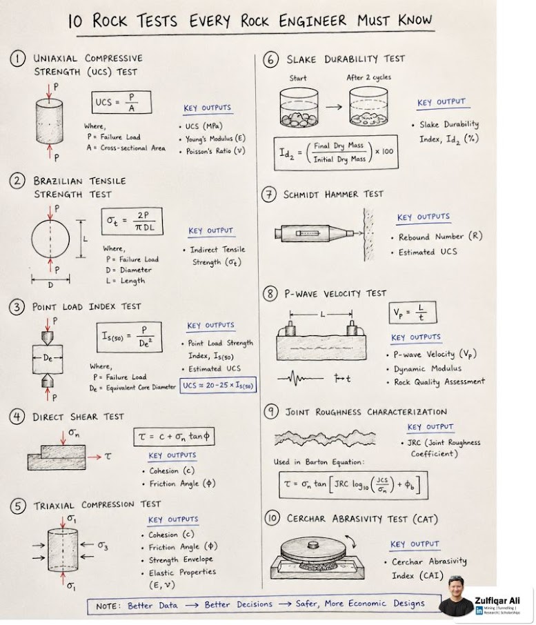
For ballast-source qualification, ballast condition surveys and subballast design, add the following to the soil program:
After Selig & Waters (1994), chs. 7, 8 and 9. Full reference under Supplemental Sources.
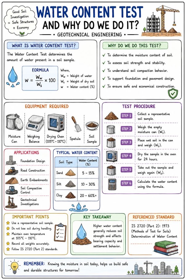
Method: Oven-dry at 230 ± 9°F for minimum 16 hours (peat and organic soils: 140°F).
Equation:
w = (M_water / M_dry) × 100%
where M_water = mass of water (mass_wet − mass_dry); M_dry = mass of dry soil.
Output: Water content w (%), dimensionless.
Minimum frequency: Every disturbed and undisturbed sample. Water content is the most fundamental test in the program — never omit it.
Reference graphics
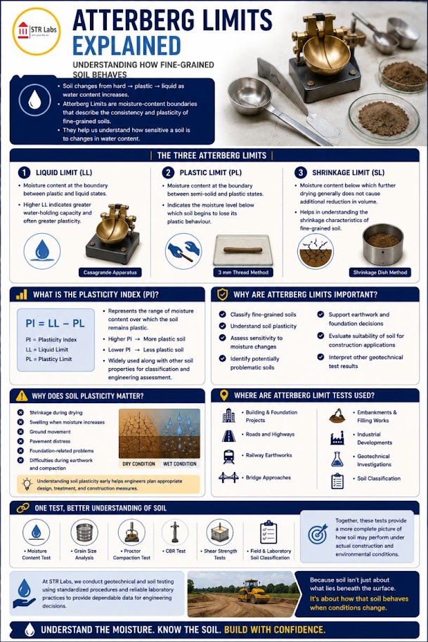
Liquid Limit (LL): Casagrande cup method; flow curve plotted; LL at N = 25 blows.
Plastic Limit (PL): ⅛-in. thread rolling on glass plate.
Plasticity Index: PI = LL − PL
Liquidity Index: LI = (w − PL) / PI
Activity: A = PI / (% < 0.002 mm)
Output: LL, PL, PI (all %); LI and A dimensionless.
Minimum frequency: 1 per fine-grained stratum per boring; 1 per 5 ft depth in highly variable fine-grained profiles.
Reference graphics
Reference graphics · click to zoom
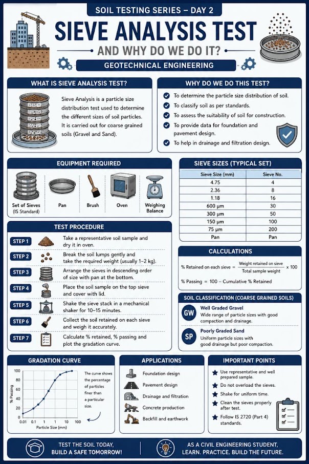
Sieve analysis (ASTM D6913): Applicable for material with particles retained on the No. 200 sieve. Sieves: 3 in., 2 in., 1½ in., 1 in., ¾ in., ½ in., No. 4, No. 10, No. 20, No. 40, No. 60, No. 100, No. 200.
Hydrometer analysis (ASTM D7928): For material passing No. 200 (clay and silt sizes). Combined with sieve for full gradation curve (ASTM D6913 + D7928).
Key outputs:
Minimum frequency: 1 per stratum per boring for classification; additional tests for filter design and liquefaction susceptibility assessment.
Reference graphics
Reference graphics · click to zoom
Method: Pycnometer (volumetric flask) method; soil displaced volume in de-aired water.
Equation:
G_s = M_sd / (M_sd + M_pw − M_spw) (dimensionless)
where M_sd = mass of dry soil; M_pw = mass of pycnometer + water; M_spw = mass of pycnometer + soil + water.
Typical values: G_s = 2.60–2.75 (mineral soils); 2.60–2.65 (clean quartz sand); 2.70–2.80 (iron-rich soils).
Minimum frequency: 1 per soil type in each project; required for void ratio and consolidation calculations.
Reference graphics
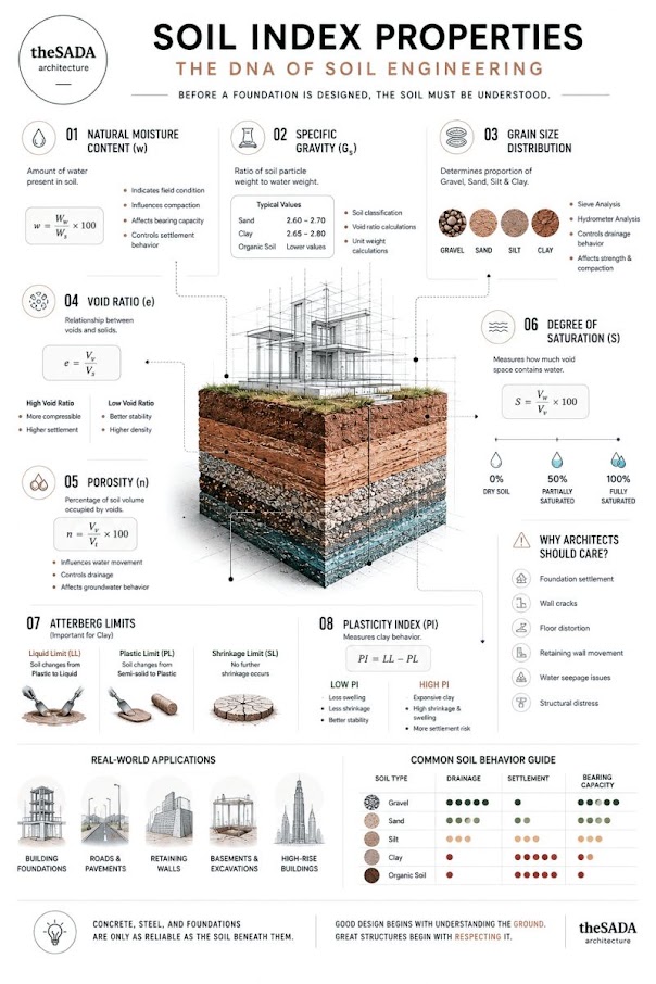
Standard Proctor (ASTM D698):
Modified Proctor (ASTM D1557):
Output: Compaction curve (γ_d pcf vs. w %); γ_d,max (pcf); w_opt (%)
Zero-Air-Voids (ZAV) line: γ_d,ZAV = G_s × γ_w / (1 + G_s × w/100) (pcf)
Minimum frequency: 1 Modified Proctor per borrow source or fill material type (not per sample); repeat if source changes during construction.
Reference graphics
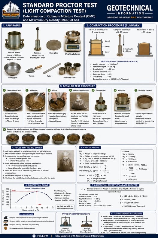
Reference graphics · click to zoom
Method: Laboratory CBR at Modified Proctor density (95% RC minimum). Specimen soaked 96 hours at Standard loading conditions.
Penetration resistance equation:
CBR = (P_sample / P_standard) × 100%
where:
Use the higher CBR from 0.1 or 0.2 in. penetration (recheck if 0.2 in. governs).
Output: CBR (%); used directly for pavement design (Chapter 18, Section 18.1).
Minimum frequency: 1 per subgrade soil type per project; 3+ tests for intermodal yard pavement design.
Reference graphics
Method: Cyclic triaxial test with conditioning sequence (500 cycles at 4 psi deviator) followed by 15 stress states per AASHTO T307 protocol.
M_r from regression (NCHRP 1-28A model):
M_r = k₁ × P_a × (θ/P_a)^k₂ × (τ_oct/P_a + 1)^k₃ (psi)
where:
Minimum frequency: Required by Amtrak for all NEC pavement subgrade investigations; recommended by BNSF for intermodal yard pavement design; 1 test per subgrade soil type.
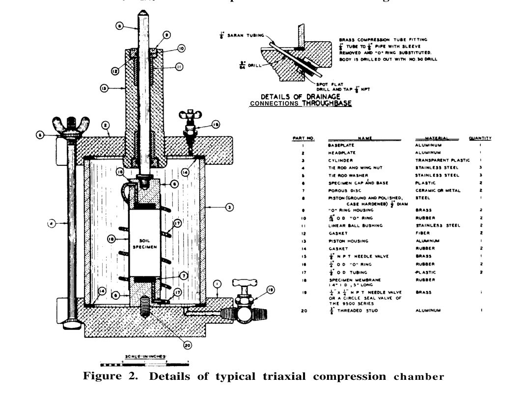
Repeated-load triaxial (or simple shear) tests give two results that matter for track:
Tiny plastic strains per cycle add up to large settlement over millions of cycles, so report both.
What to look for.
Test conditions. Test at the field moisture and density, including a wet-of-optimum case (Chapter 18, §18.2.2). Fine-grained modulus falls steeply on the wet side.
After Selig & Waters (1994), chs. 3, 7 and 10. Full reference under Supplemental Sources.
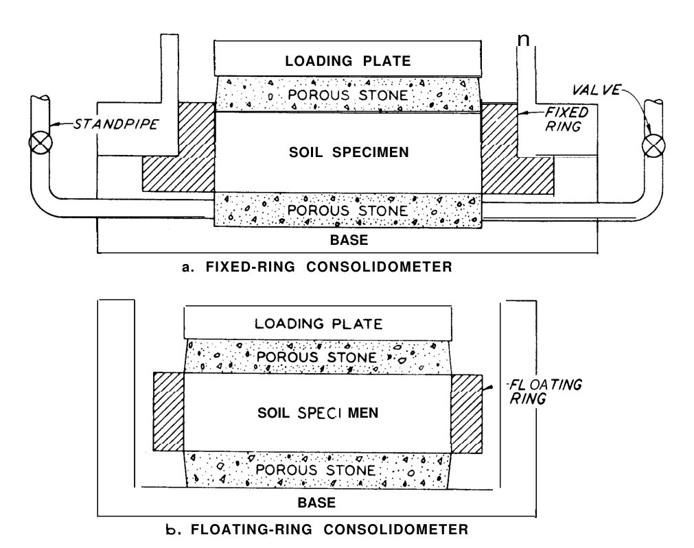
Method A: Incremental load; load doubling each 24-hour interval; loads: 125–250–500–1,000–2,000–4,000–8,000 psf (standard); extend to 16,000 psf for deep or heavily preloaded sites.
Method B: Constant rate of strain (CRS); continuous loading at a controlled strain rate.
Key outputs (English units):
| Parameter | Symbol | Units | Equation |
|---|---|---|---|
| Compression index | C_c | dimensionless | Slope of e-log σ'_v curve (NC range) |
| Recompression index | C_r | dimensionless | Slope of e-log σ'_v curve (OC range); ≈ C_c/5 to C_c/10 |
| Preconsolidation pressure | σ'_p | tsf | Casagrande graphical construction |
| OCR | — | dimensionless | σ'_p / σ'_v0 |
| Coefficient of consolidation | c_v | ft²/day | c_v = T_v × H_dr² / t (see Chapter 12) |
| Secondary compression index | C_α | dimensionless | Δe / Δ log t (secondary range) |
Minimum frequency: 1 per fine-grained stratum per project; minimum 3 tests in any stratum requiring settlement analysis.
Reference graphics
Reference graphics · click to zoom
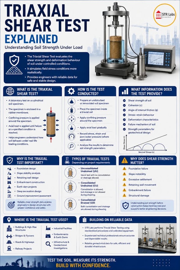
Method: Undrained shear test on undisturbed sample; three specimens at different confining pressures (typically 500, 1,000, 2,000 psf); no drainage allowed during shear.
Output: s_u (psf or tsf) from Mohr circle at failure; φ_u ≈ 0° for saturated clay.
Note: For saturated clay, UU test gives s_u directly regardless of confining pressure — the Mohr circle diameter is constant. UU is appropriate for short-term (undrained) stability analysis only.
Minimum frequency: 1 per soft or medium clay stratum per boring at critical cross-sections (slope stability, embankment loading over soft clay).
Reference graphics
Reference graphics · click to zoom
After Selig & Waters (1994), ch. 3. Full reference under Supplemental Sources.
Method: Specimens consolidated to two or three effective confining pressures (σ'₃); sheared undrained with pore pressure measurement; effective stress Mohr circles give c' and φ'.
Output: c' (psf), φ' (degrees) — effective strength parameters for long-term (drained) analysis.
Minimum frequency: Required for all critical slope stability analyses (NSR clay shale, CPKC prairie clay, CN sensitive marine clay); 1 set (3 specimens) per stratum per project minimum.
Reference graphics
Reference graphics · click to zoom
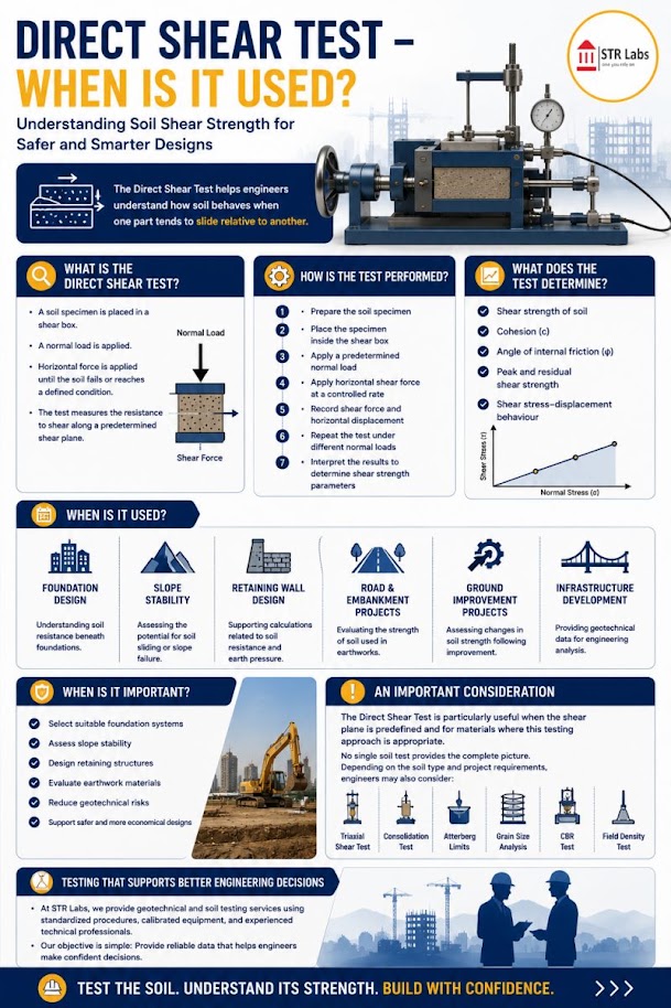
Method: Specimen sheared at constant normal stress; three tests at different normal stresses.
Peak and residual strength:
τ_peak = c' + σ_n × tan φ'_peak (psf)
τ_residual = σ_n × tan φ'_r (psf, c' = 0 for residual)
Output: c' (psf), φ' (degrees), φ'_r (degrees).
Use cases: Residual strength for CPKC clay shale and NSR weathered shale slope stability; rock joint shear strength for cut slope design.
Minimum frequency: 1 per stratum requiring residual strength parameters; rock joints: minimum 3 direct shear tests per joint set per project.
Reference graphics
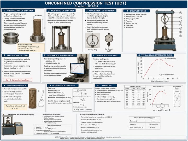
Method: Axial loading to failure at unconfined conditions (σ₃ = 0). Quick and inexpensive.
Output: q_u (psf or tsf); s_u = q_u / 2.
Limitation: UU triaxial provides more reliable s_u; unconfined compression can underestimate s_u in fissured or brittle clays. Use for screening; not for final design in critical applications.
Minimum frequency: Appropriate for routine s_u checks on Shelby tube samples; supplement with UU triaxial for design-level analysis.
Reference graphics
Constant head (ASTM D2434): For coarse-grained soils (k > 10⁻³ ft/day).
k = (Q × L) / (A × h × t) (ft/day)
where Q = flow volume (ft³); L = specimen length (ft); A = cross-sectional area (ft²); h = head differential (ft); t = test duration (day).
Flexible wall permeameter (ASTM D5084): For fine-grained soils (k < 10⁻³ ft/day).
k = (a × L × ln(h₁/h₂)) / (A × t) (ft/day)
where a = standpipe area (ft²); L = specimen length (ft); h₁, h₂ = head at start and end; t = elapsed time (day).
Minimum frequency: 1 per stratum for drainage design; 3 per stratum for seepage analysis through embankments or dams.
Reference graphics
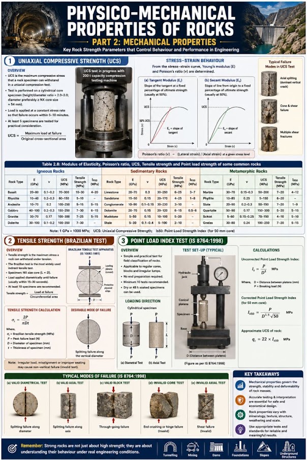
Method: Rock core or irregular lump loaded to failure between conical platens.
Point load strength index:
I_s = P / D_e² (psi or psf)
where P = failure load (lb); D_e = equivalent core diameter (in.).
Size-corrected index:
I_s(50) = F × I_s where F = (D_e/1.97 in.)^0.45
Estimated UCS of rock:
q_u(rock) ≈ 24 × I_s(50) (psi) [Broch & Franklin 1972; I_s in psi]
Minimum frequency: Minimum 5 specimens per rock type per project; not a substitute for UCS testing for critical rock foundation designs.
Reference graphics
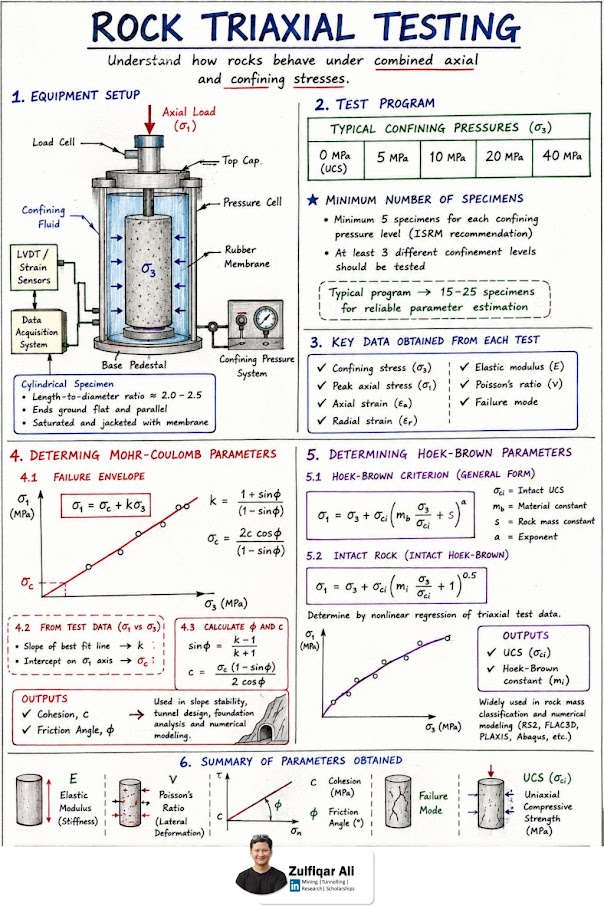
USACE manuals (EM 1110-2-1902 slope stability, EM 1110-2-2504 sheet piles, and others cited in this manual) use letter names for the basic triaxial tests: Q = unconsolidated-undrained (UU); R = consolidated-undrained (CU); S = consolidated-drained (CD), which is also the long-term drained case. The Q test applies only to soils that are not free-draining, and R-test specimens should generally be fully saturated before shear. Errors EM 1110-2-1906 lists for R tests: back-pressure increments too large or applied too fast; chamber and back pressure not held precisely (which can overconsolidate the specimen); shearing before consolidation is complete; too fast a strain rate; temperature drift; and water absorbed from the porous inserts after the test, which biases the final water content. For S tests the main errors are strain rate and volume-change measurement. In pervious soils, water redistributes even in a quick Q test, so measure the water content of the middle third separately from the ends.
Section 10.3.8 gives cv = TvHdr2/t but not how t is found. The two standard curve-fitting methods (Das lab manual) are:
With double drainage, Hdr is half the average specimen height during the increment. Report which method was used. The two methods commonly give different cv values for the same increment, and the report should say which one the settlement-time analysis in Chapter 12 used.
Source: U.S. Army Corps of Engineers (1970, with changes). Laboratory Soils Testing. EM 1110-2-1906 · Das, B. M. (2002). Soil Mechanics Laboratory Manual, 6th ed. Oxford University Press
Railroad cuts in Appalachian and prairie shales (Chapter 13) need durability as well as strength data, and Atterberg limits of clay shale depend on how the sample was processed. EM 1110-2-1906 therefore standardizes three preparations: blenderized (the primary reference — dried below 122°F at < 30% RH, soaked at least 48 hr, then blended as a slurry above 300% water content or twice the LL); undried (shaved directly into distilled water); and air-dried (one drying–soaking cycle). The spread among the three indicates the strength of interparticle bonds. Report which method produced the limits used for design.
Slake durability (Franklin and Chandra, 1972; ASTM D4644): oven-dried rock lumps are rotated for 10 minutes in a sieve-mesh drum half immersed in 68°F water. Id is the percentage of the initial dry mass retained. Nagaraj reports reproducibility within 5% at 95% confidence, and the test discriminates well between mudstones that otherwise look alike.
| Id (%) | 0–25 | 25–50 | 50–75 | 75–90 | 90–95 | 95–100 |
|---|---|---|---|---|---|---|
| Durability | Very low | Low | Medium | High | Very high | Extremely high |
After Franklin and Chandra (1972). As printed in Nagaraj’s Table 9.7, the 75–90 and 90–95 labels are transposed; the order shown here is the original.
For clay shales, Nagaraj also reproduces the Morgenstern and Eigenbrod (1974) classification, which combines the amount of slaking (by the liquid limit of the slaked material: < 20 very low to > 140 very high) with the rate (change in liquidity index in the first cycle: < 0.75 slow, 0.75–1.25 fast, > 1.25 very fast). Add slake durability to the rock column of Table 10-1 for every cut in shale, mudstone or claystone and for any rock proposed as riprap or fill.
Source: U.S. Army Corps of Engineers (1970, with changes). Laboratory Soils Testing. EM 1110-2-1906 · Nagaraj, T. S. (1993). Principles of Testing Soils, Rocks and Concrete. Elsevier (Developments in Geotechnical Engineering)
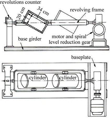
| Test | Equipment and procedure | Result |
|---|---|---|
| Deval (1896) | 11-lb sample in cylinders 8 in. dia. × 13 in., inclined 30°; 10,000 revolutions at 2,000 rev/h (about 5 h); dry or wet | Deval coefficient from % attrition. Typical minimums: > 12 (limestone), > 14 (hard rock), some railways > 16 |
| Los Angeles (1926) | Drum 28 in. dia. × 20 in.; 11-lb sample with 12 steel balls of 15 oz each; 500 revolutions at 30–33 rpm (about 15 min). EN version: 22-lb sample, 1,000 revolutions | % passing No. 12 (French) or No. 8 (British) sieve. Many specifications: LA < 25. EN reference test |
| Micro-Deval | 1.1 lb of ⅜–½ in. gravel, one 11-lb steel ball and 2.6 qt of water in an 8-in. cylinder; 12,000 revolutions at 100 rpm. EN version: 22 lb, 14,000 revolutions | MDE = % finer than No. 12. Used mainly for subballast; subballast MDE < 15–20 |
North American ballast specifications (AREMA Chapter 1) use the ASTM Los Angeles test for large coarse aggregate (ASTM C535). Results from the European methods are not interchangeable with ASTM results without correlation.
Cyclic behavior. Ballast takes a large permanent set on first loading as stones rearrange, then accumulates strain slowly: εN = ε1(1 + c·log N), with c ≈ 0.2 (European ORE and British Rail research) or 0.25–0.40 (American research). On that basis it takes 100,000–300,000 cycles to double the first-cycle plastic strain. Ballast modulus roughly doubles over the first 1,000 cycles and then stays nearly constant; gravel subballast modulus does not change with cycles. Repeated-load triaxial programs should run long enough to get past this initial bedding-in.
Figures · click to zoom
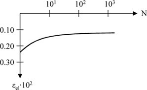
After Profillidis (2014), §12.3–12.4, Eq. 12.1, Figs. 12.3–12.4. Full reference under Supplemental Sources.
| Test | Standard | What it gives |
|---|---|---|
| Atterberg limits | ASTM D4318 | Liquid limit, plastic limit, plasticity index; classifies fines |
| Particle-size distribution | ASTM D422 | Sieve gradation, % finer than No. 200, hydrometer split of silt and clay |
| Moisture content | ASTM D4643 | Water content by drying |
| Unconfined compressive strength | ASTM D2166 | Direct strength of cohesive samples |
| Proctor compaction | ASTM D698 / D1557 | Target density and optimum moisture for fill and subgrade |
Compaction can roughly double a soil’s strength. The fines content of granular fill controls its drainage, frost susceptibility and strength after rain, so specify and test fines on ballast and sub-ballast deliveries rather than accepting material that only looks good dry.
Figures · click to zoom
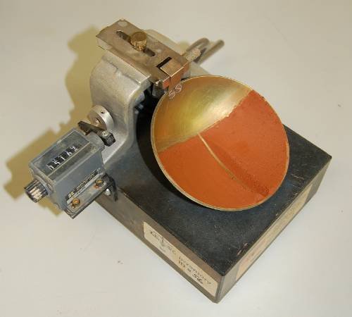
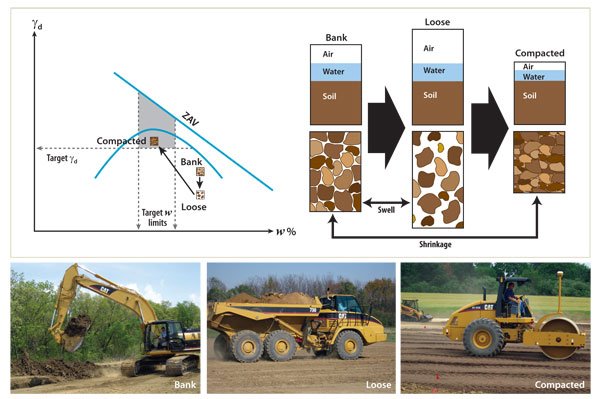
After Geotechnology for Railroaders Program, Module 2; §09–10. Full reference under Supplemental Sources.
Case study: 10.16.1 Curing time changes compaction and CBR results (Look 2023), in §10.16 Case Studies.
Shelby tubes (ASTM D1587 thin-wall samples) must be:
Sample Quality Designation (Lunne et al. 1997) — referenced in Chapter 6:
| Δe/e₀ | Quality |
|---|---|
| < 0.04 | Very good to excellent |
| 0.04–0.07 | Good to fair |
| 0.07–0.14 | Poor |
| > 0.14 | Very poor |
Report SQD for all consolidation and triaxial test specimens. UPRR and BNSF Engineering Instructions require that samples with SQD = Poor or Very Poor be noted in the report with a corresponding caveat on the reliability of strength and compressibility parameters derived from them.
Reference graphics
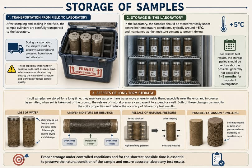
A chain of custody (COC) form must accompany every sample shipment from field to laboratory. Required fields:
CSXT and Amtrak require COC forms to be scanned and submitted with the laboratory report as a QC attachment.
A minimum of 10% of all tests (by test type) must be run in duplicate as a QC check. Duplicate tests are run on split halves of the same sample by the same method. Acceptable precision limits:
| Test | Acceptable Duplicate Difference | Action if Exceeded |
|---|---|---|
| Water content (D2216) | ≤ 1.0% | Repeat test on third portion |
| Atterberg limits (D4318) | LL ≤ 2%, PL ≤ 2% | Repeat; average of three if still outside |
| Modified Proctor (D1557) | γ_d,max ≤ 1.0 pcf; w_opt ≤ 1.0% | Rerun entire compaction curve |
| Consolidation C_c (D2435) | ≤ 0.05 | Flag and report; use higher value for design |
| UU triaxial s_u (D2850) | ≤ 10% of mean | Investigate specimen preparation |
| CBR (D1883) | ≤ 5 percentage points | Average of three specimens |
The laboratory must maintain certified reference standards for:
Each laboratory report must contain:
Specimen selection matters more than test count. EM 1110-2-1906 stresses that strength, compressibility and permeability can vary severalfold within a few inches. Specimen selection therefore needs personal inspection of the samples by the laboratory and the design engineer together, not selection from boring logs alone. Its guiding principle: “one good test is not only far better than many poor tests, but is also less expensive.” Undisturbed samples should not be stored for long periods, because physical and chemical changes eventually invalidate them.
Source: U.S. Army Corps of Engineers (1970, with changes through 1986). Calibration of Laboratory Soils Testing Equipment. EM 1110-2-1909 · U.S. Army Corps of Engineers (1970, with changes). Laboratory Soils Testing. EM 1110-2-1906
Case study: 10.16.2 Laboratory variation in Cooroy clay compaction curves (Look 2023), in §10.16 Case Studies.
| Test | CSXT | NSR | UPRR | BNSF | CPKC | Amtrak | CN | G&W |
|---|---|---|---|---|---|---|---|---|
| Water content, Atterberg, grain size | 5 business days | 5 business days | 5 business days | 5 business days | 5 business days | 5 business days | 5 business days | 5 business days |
| Modified Proctor | 7 business days | 7 business days | 7 business days | 7 business days | 7 business days | 7 business days | 7 business days | 7 business days |
| CBR (soaked) | 10 business days | 10 business days | 10 business days | 10 business days | 10 business days | 10 business days | 10 business days | 10 business days |
| UU Triaxial | 10 business days | 10 business days | 10 business days | 10 business days | 10 business days | 10 business days | 10 business days | 10 business days |
| CU Triaxial | 15 business days | 15 business days | 15 business days | 15 business days | 15 business days | 15 business days | 15 business days | 15 business days |
| Consolidation (D2435) | 14 business days | 14 business days | 14 business days | 14 business days | 14 business days | 14 business days | 14 business days | 14 business days |
| Resilient modulus (T307) | Not required | Not required | Not required | 15 business days | 15 business days | 15 business days | 15 business days | Not required |
Rush processing (1.5–2× standard fee): available from most accredited labs at 50–70% of standard turnaround times. Confirm availability at project initiation for emergency and fast-track projects.
| Railroad | Untested disturbed samples | Tested Shelby tubes | Rock cores | Ballast samples | Governing Std. |
|---|---|---|---|---|---|
| CSXT | 90 days post-report | 1 year post-report | 1 year post-report | 90 days | CSXT Eng. Std. |
| NSR | 90 days post-report | 1 year post-report | 1 year post-report | 90 days | NSR Eng. Std. |
| UPRR | 6 months post-report | 2 years post-report | 2 years post-report | 6 months | UPRR Eng. Instr. Manual |
| BNSF | 6 months post-report | 2 years post-report | 2 years post-report | 6 months | BNSF Eng. Instructions |
| CPKC | 6 months post-report | 2 years post-report | 2 years post-report | 6 months | CPKC Track Standards |
| Amtrak | 1 year post-report | 3 years post-report | 3 years post-report | 1 year | Amtrak Eng. Std. |
| CN | 6 months post-report | 2 years post-report | 2 years post-report | 6 months | CN Eng. Standards |
| G&W | 90 days post-report | 1 year post-report | 1 year post-report | 90 days | G&W Eng. Bulletin |
All nine client railroads reserve the right to request sample re-testing or third-party verification testing within the retention period.
| Railroad | Required Accreditation | Scope Verification | Submission Required |
|---|---|---|---|
| CSXT | AASHTO Accreditation Program (AAP) or CCRL | Per-method scope | Yes — with lab report |
| NSR | AAP or CCRL | Per-method scope | Yes |
| UPRR | AAP or A2LA | Per-method scope | Yes |
| BNSF | AAP or A2LA | Per-method scope | Yes |
| CPKC | AAP (US territory); SCC (Canadian territory) | Per-method scope | Yes |
| Amtrak | AAP or A2LA; CCRL for NEC | Per-method scope | Yes |
| CN | AAP (US territory); SCC or BNQ (Canadian territory) | Per-method scope | Yes |
| G&W | AAP preferred; CCRL accepted | Not required | On request |
Key accreditation bodies:
Project context: CSXT Georgia Division bridge approach embankment. Consolidation test on Shelby tube sample from B-3 at 18–20 ft depth (soft gray kaolin clay, CH).
Lab data (at end of each load stage):
| σ'_v (tsf) | Void ratio e |
|---|---|
| 0.125 | 1.820 |
| 0.250 | 1.795 |
| 0.500 | 1.762 |
| 1.000 | 1.698 |
| 2.000 | 1.590 |
| 4.000 | 1.430 |
| 8.000 | 1.235 |
| 16.000 | 1.015 |
Step 1: Identify σ'_p (Casagrande graphical method)
From the e-log σ'_v plot (described graphically):
Step 2: Compute C_c (NC range, 2.0–8.0 tsf)
C_c = Δe / Δ(log σ'_v) = (1.590 − 1.235) / (log 8.0 − log 2.0)
= 0.355 / (0.903 − 0.301) = 0.355 / 0.602 = 0.590
Step 3: Compute C_r (OC range, 0.125–1.0 tsf)
C_r = (1.820 − 1.698) / (log 1.000 − log 0.125)
= 0.122 / (0 − (−0.903)) = 0.122 / 0.903 = 0.135
Step 4: OCR
Current effective overburden: σ'_v0 = (γ_sat − γ_w) × z = (115 − 62.4) pcf × 19 ft = 999 psf = 0.50 tsf
OCR = σ'_p / σ'_v0 = 1.50 / 0.50 = 3.0
Conclusion: Moderately OC clay. Use Chapter 12 OC settlement equations for this stratum (Eq. 7-6 below σ'_p; Eq. 7-7 if stress path crosses σ'_p). Report C_c = 0.590, C_r = 0.135, σ'_p = 1.50 tsf, OCR = 3.0 in the engineering properties table (Table 5 of the GDR/FGR).
Project context: BNSF Kansas City intermodal yard expansion. Subgrade soil is lean clay (CL); Modified Proctor performed to establish compaction reference, followed by soaked CBR at 95% RC.
Modified Proctor results:
| Water Content w (%) | γ_d (pcf) |
|---|---|
| 10.5 | 111.8 |
| 12.0 | 115.4 |
| 14.0 | 118.2 |
| 16.0 | 117.1 |
| 18.0 | 113.5 |
Step 1: Identify γ_d,max and w_opt
Peak dry density: γ_d,max = 118.2 pcf at w_opt = 14.0%
Step 2: Target density for CBR specimen
γ_d,target = 0.95 × 118.2 = 112.3 pcf (at 95% RC per BNSF Engineering Instructions)
Step 3: CBR test results at 0.1 in. penetration
Measured load: P_sample = 730 lb; P_standard = 3,000 lb
CBR = (730 / 3,000) × 100% = 24.3%
At 0.2 in. penetration: P_sample = 960 lb; P_standard = 4,500 lb
CBR(0.2) = (960 / 4,500) × 100% = 21.3%
0.1 in. governs: Design CBR = 24.3%
Step 4: Design interpretation
Per Chapter 18, Table 10-1, CBR = 24.3% → Fair subgrade (CBR 20–50 range). BNSF Engineering Instructions require CBR ≥ 20% for intermodal yard pavement subgrade or blanket layer to achieve this. Subgrade marginally adequate; recommend confirming with ≥ 3 CBR tests across the yard footprint.
Project context: NSR Appalachian Division cut slope in residual silty clay (CL-ML). CU triaxial test with pore pressure measurement on three specimens.
Test results:
| Specimen | σ₃ (psf) | Δu at failure (psf) | q = (σ₁−σ₃)/2 (psf) | p = (σ₁+σ₃)/2 (psf) |
|---|---|---|---|---|
| A | 1,000 | 400 | 820 | 1,820 |
| B | 2,000 | 710 | 1,540 | 3,540 |
| C | 3,000 | 1,050 | 2,290 | 5,290 |
Effective stress parameters:
| Specimen | σ'₃ = σ₃ − Δu (psf) | σ'₁ = σ₃ + 2q − Δu (psf) |
|---|---|---|
| A | 600 | 2,240 |
| B | 1,290 | 4,370 |
| C | 1,950 | 6,530 |
Step 1: Plot Mohr circles in effective stress space (described):
Circle A: center = (600+2240)/2 = 1,420; radius = (2240−600)/2 = 820 Circle B: center = (1290+4370)/2 = 2,830; radius = (4370−1290)/2 = 1,540 Circle C: center = (1950+6530)/2 = 4,240; radius = (6530−1950)/2 = 2,290
Step 2: Fit Mohr-Coulomb envelope
Using linear regression on (p', q') pairs: slope = sin φ' = (2,290−820)/(4,240−1,420) × (rise/run from regression)
For this dataset (simplified): sin φ' ≈ 0.517 → φ' = 31°
c' intercept ≈ 200 psf (from y-intercept of fitted line)
Step 3: Report
Effective friction angle: φ' = 31°, effective cohesion: c' = 200 psf
Per NSR Engineering Standards Manual, these parameters apply to long-term (drained) slope stability analysis. NSR requires a minimum of two additional specimens for confirmation before finalizing parameters for critical cut slope designs (FS < 1.3 zone).
| Boring | Sample | Depth (ft) | USCS | LL | PL | PI | w (%) | γ_d (pcf) | s_u (tsf) | φ' (°) | c' (psf) | C_c | C_r | σ'_p (tsf) | k (ft/day) |
|---|---|---|---|---|---|---|---|---|---|---|---|---|---|---|---|
| B-1 | SS-3 | 8–10 | CL | 42 | 20 | 22 | 24.1 | — | — | — | — | — | — | — | — |
| B-1 | ST-1 | 12–14 | CH | 65 | 28 | 37 | 38.5 | 78.2 | 0.24 | — | — | 0.52 | 0.11 | 1.20 | — |
| B-2 | SS-4 | 10–12 | ML | 35 | 22 | 13 | 18.2 | — | — | — | — | — | — | — | — |
| B-3 | ST-1 | 18–20 | CH | 71 | 29 | 42 | 42.1 | 76.5 | 0.19 | — | — | 0.59 | 0.14 | 1.50 | 2.1×10⁻⁵ |
| B-3 | SS-6 | 25–27 | SC | — | — | 4 | 9.8 | — | — | 32° | 0 | — | — | — | — |
| B-4 | ST-2 | 15–17 | CL | 48 | 22 | 26 | 29.4 | 80.1 | 0.31 | — | — | 0.44 | 0.09 | 1.35 | — |
| B-5 | SS-3 | 8–10 | CL | 44 | 21 | 23 | 22.8 | — | — | — | — | — | — | — | — |
| B-6 | ST-1 | 12–14 | CH | 68 | 27 | 41 | 40.2 | 77.4 | 0.22 | 31° | 200 | 0.57 | 0.12 | 1.45 | — |
Reference graphics
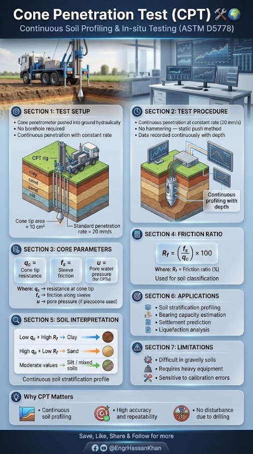
Checklist · Part V · Subsurface Exploration
Pre-Field
Field
Laboratory Phase
Report Integration
| Topic | See Also |
|---|---|
| SPT N-value correction using γ_d and G_s | Chapter 6 |
| In situ test correlation to lab parameters | Chapter 7 |
| USCS classification using Atterberg limits and grain size | Chapter 8 |
| Groundwater (effect on consolidation parameters) | Chapter 9 |
| Bearing capacity using c', φ' from triaxial | Chapter 11 |
| Settlement using C_c, C_r, σ'_p from consolidation | Chapter 12 |
| Slope stability using φ' and c' from CU triaxial | Chapter 13 |
| Liquefaction using fines content and FC correction | Chapter 14 |
| CBR and M_r for pavement design | Chapter 18 |
| Ground improvement parameter selection | Chapter 17 |
| Retaining wall backfill φ' from direct shear | Chapter 16 |
| Subgrade s_u from UU triaxial for subgrade FS | Chapter 2 |
| Reference Proctor for compaction acceptance | Chapter 15 |
| Lab data table format in final report | Appendix E |
| Lab test data table template (blank) | Appendix B |
Q1. A consolidation test data set shows the following e-log σ'_v values: at σ'_v = 1.0 tsf, e = 1.42; at σ'_v = 4.0 tsf, e = 1.18. The current effective overburden is σ'_v0 = 0.80 tsf and the Casagrande graphical construction gives σ'_p = 1.60 tsf. Calculate: (a) C_c in the NC range, (b) OCR, and (c) which settlement equation from Chapter 12 applies (NC equation, OC below σ'_p, or OC crossing σ'_p)?
Answer:
Q2. A nuclear gauge reads γ_d,field = 117.4 pcf on a fill material. The Modified Proctor gives γ_d,max = 120.5 pcf. (a) What is RC%? (b) Does this pass CSXT's 95% requirement? (c) The moisture content is 17.2% vs. w_opt = 14.0%. Is the moisture within CSXT's ±3% tolerance?
Answer:
Q3. Two Shelby tube samples from the same stratum undergo consolidation testing. Sample A gives C_c = 0.45 with SQD "Good to Fair" (Δe/e₀ = 0.06). Sample B gives C_c = 0.31 with SQD "Poor" (Δe/e₀ = 0.12). Which value should be used for design and why?
Answer: Use C_c = 0.45 from Sample A. Sample B's SQD of "Poor" indicates significant sample disturbance during sampling, transport, or extrusion. Disturbance generally artificially reduces apparent stiffness in the early part of the consolidation curve, leading to an underestimated C_c — which would underestimate settlement and produce an unconservative design. Sample A, rated "Good to Fair," provides the more reliable result. Document in the report that Sample B's result was rejected due to poor quality (Lunne et al. 1997 SQD criteria) and that C_c = 0.45 governs settlement calculations for this stratum.
Q4. A CU triaxial test on three specimens gives peak deviator stresses (σ₁ − σ₃) at failure of 1,840 psf, 3,280 psf, and 4,920 psf at confining pressures of 1,000, 2,000, and 3,000 psf respectively. Pore pressures at failure are 450, 820, and 1,200 psf. Calculate: (a) σ'₃ for each specimen, (b) σ'₁ for each specimen, and (c) estimate φ' from the ratio of radii to centers.
Answer:
Q5. A soaked CBR specimen gives the following load-penetration data: at 0.1 in. — 880 lb; at 0.2 in. — 1,260 lb. The zero-load reading showed 15 lb due to seating. (a) Correct the loads. (b) Calculate CBR at 0.1 in. and 0.2 in. (c) Report the design CBR.
Answer:
Field case studies by Burt G. Look, from Earthworks: Theory to Practice – Design and Construction (CRC Press/Balkema, 2023), chosen for this chapter’s topics. Each is summarized from the book with its key figures and a closing note on railroad application added by the authors of this manual. Credit for the case material belongs to Look; see item S8 under Supplemental Sources.
Related section: 10.3 Test Methods — ASTM Standards and English Unit Outputs
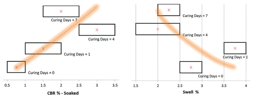
Samples of Bundamba clay (plasticity index 47%, 97% passing No. 40, 69%–82% fines) were cured for 0, 1, 4 and 7 days before compaction and soaked and unsoaked CBR testing:
For railroad work: plastic clay subgrade samples for CBR, resilient modulus or Proctor testing should be cured to the period the test standard requires, and the curing time should be reported. A test turned around too quickly can push the design either way.
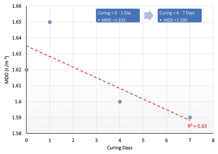
Source: Look, B. G. (2023). Earthworks: Theory to Practice – Design and Construction. CRC Press/Balkema. Case study §5.8, pp. 142. Summarized and paraphrased; figures reproduced for internal reference. Full reference under Supplemental Sources.
Related section: 10.5 Laboratory QA/QC
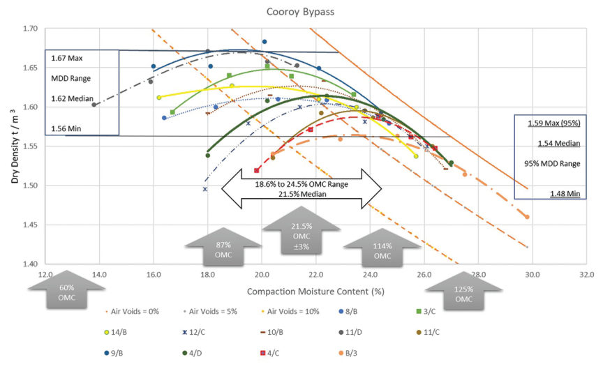
Eleven standard compaction tests on clay from one project site at Cooroy, Queensland (55 compaction points) gave maximum dry densities from 97–104 pcf, median 1.62, and optimum moisture contents from 18.6% to 24.5%, median 21.5%. The idea of a unique MDD and OMC does not hold for clays. The repeatability allowed in the Australian standard suggests 85%–115% of OMC as a realistic moisture window, yet many specifications ask for ±2% of OMC, which testing variation alone makes unachievable.
The real target is low air voids: much below 85% of OMC, air voids exceed about 10%. Look also warns that the compacted soil will not stay at its placement moisture, so the moisture target should guide field effort and not be a pass/fail criterion. Density is the pass/fail measure. Compaction well above MDD or dry of OMC raises suction, so the “stronger” material is more sensitive to later moisture change.
For railroad work: the ±2% moisture band suits processed granular materials such as subballast, not high-moisture clays in embankment or subgrade. Use a band that reflects the laboratory’s own repeatability.
Source: Look, B. G. (2023). Earthworks: Theory to Practice – Design and Construction. CRC Press/Balkema. Case study §7.9, pp. 230–232. Summarized and paraphrased; figures reproduced for internal reference. Full reference under Supplemental Sources.
Authors: Daniel P. Colwell and Mario Ruel. This chapter was written and compiled by Daniel P. Colwell and Mario Ruel for Railway Ground Hazard Risk Management.
Technical content is drawn from the published sources below, and credit for that material belongs to their authors and publishers. Tables, equations and figures taken from a specific source are also cited where they appear.
File locations for these documents are listed under Supplemental Sources — LEVI Library.
Material in the green “Supplemental reference” boxes throughout this chapter was added from the following documents in the LEVI geotechnical library. Text is summarized or paraphrased; tables are reproduced with their original source noted; figures are reproduced from the cited document for internal reference use. Consult the original document before relying on a value for design. Blocks marked “After Selig & Waters (1994)” summarize item S7 for railroad clients; tables are condensed from the book and its figures are not reproduced. The Case Studies section summarizes case studies from item S8 by Burt G. Look; its figures are reproduced from the book for internal reference use, and the closing “For railroad work” note in each case study is added by the authors of this manual.