
Geotechnical engineering libraryContact
Formerly Geo Rail Chapter 13 — Railroad Track Subgrade: Special Topics
Geotechnical Services Manual for Railroad Clients
A Consultant's Reference for Delivering Geotechnical Engineering Services Across North American Railroad Capital Programs
Apps on dirtbert.com that support this chapter. Each one runs in a web browser on a desktop or a phone, with nothing to install. How to use the apps (I.3).
NANCY pages ask you to accept the Use and Disclaimers once in each browser. MINA is a monitoring aid and is not for operational dispatch decisions.
The track subgrade is the engineered foundation upon which the entire superstructure — rail, ties, ballast, and subballast — rests. Unlike highway or airfield pavement subgrades, railroad subgrades are subjected to high-frequency, high-magnitude cyclic loading from heavy-axle freight traffic (286,000 lb gross rail load is the North American standard), combined with dynamic amplification, repeated wetting and drying, freeze-thaw action, and the progressive accumulation of ballast fines over time. Subgrade failures — progressive shear failure, ballast pocket formation, pumping, differential frost heave — are among the most common and expensive maintenance problems faced by North American freight railroads.
This chapter provides the geotechnical consultant's framework for characterizing, designing, and remediating railroad track subgrades. It covers the Talbot load distribution method, stress at top of subgrade, ballast and subballast specification per AREMA Manual for Railway Engineering Chapter 1, blanket layer design, subgrade failure mode identification, track modulus, ballast fouling index, subgrade drainage, and ground-penetrating radar (GPR) as a diagnostic tool. All nine client railroads — CSXT, NSR, G&W, UPRR, BNSF, CPKC, Amtrak, and CN — have specific subgrade requirements that are integrated throughout.
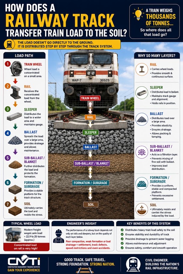
The railroad track structure transmits wheel loads through a layered system:
Rail → Tie (Crosstie) → Ballast → Subballast → Subgrade
The geotechnical consultant is primarily responsible for the subgrade and subballast layers, but must understand the full load path to correctly compute stress at the top of subgrade and specify appropriate materials.
Reference graphics
| Layer | Material | Primary Function |
|---|---|---|
| Rail | 115–141 RE steel | Carry and distribute wheel load longitudinally |
| Tie (Crosstie) | Concrete or timber, 8.5 ft long | Distribute rail load to ballast; maintain gage |
| Ballast | Crushed stone (AREMA No. 4 or No. 24) | Distribute tie load; drain; damp vibration; resist movement |
| Subballast | Granular filter/transition material | Drainage; frost protection; separate ballast from subgrade |
| Subgrade | Native or engineered fill | Ultimate load-bearing platform |
AREMA MRE Chapter 1 governs ballast and subballast specification for all nine client railroads, with client-specific supplements as noted below.
Reference graphics
Selig and Waters divide the track at the tie–ballast interface. Rail, fastenings and ties make up the superstructure. Ballast, subballast and subgrade make up the substructure. The substructure gets less attention, but its properties vary far more and are harder to define, and it drives a large share of track maintenance cost.
Ballast zones. Describe and sample each zone separately:
“Boxing” is the cribs plus the upper shoulders. A clean crib tells you nothing about the bottom ballast.
What the subballast has to do. The book lists seven functions:
Functions 3 to 5 are the “blanket” functions. Expect track built without subballast to need high maintenance. Stabilized soil, asphalt and geosynthetics can stand in for some of these functions, but not all of them (§2.4; Chapter 17).
How deep the subgrade matters. Train-induced stress is significant to about 16 ft below the bottom of tie. Model studies show that rail deflection is still about half the surface value 80 in. down. The subgrade therefore controls much of the track’s resilience even where stress has dropped off. Set trackbed boring and CPT depths to match (Chapter 5).
Ballast gradation changes in service. Three things change it:
A specification for clean new ballast only covers its condition on day one.
After Selig & Waters (1994), chs. 1, 2 and 5. Full reference under Supplemental Sources.
The AAR Heavy Axle Load program (from 1988, with testing at FAST, Pueblo) led the industry to accept 286,000-lb gross-weight cars in interchange in 1991. By 2010, nearly all coal and about 30% of general freight moved in 286k cars (about 40% of all traffic), and net benefits were about $6 billion from 1994 to 2010. The earlier move to 100-ton (263k) cars in the 1970s had “caused havoc” with track that was adequate for 70-ton cars, and rail fatigue life on tangent track fell from about 580 MGT under mixed freight to 267 MGT under 100-ton unit trains. Phase II economic studies predicted that 286k operation would raise life-cycle costs for rail, ties, ballast and subgrade, turnouts and bridges, mainly through maintenance rather than capital cost:
Table 2-S1. Predicted cost relative to 263k operation (HAL Phase II, Hargrove et al., 1996)
| West 286k (80 MGT) | West 315k | East 286k (30 MGT) | East 315k | |
|---|---|---|---|---|
| Track maintenance | 111.3% | 132.7% | 122.6% | 147.5% |
| Track capital | 102.6% | 108.6% | 106.5% | 110.0% |
| Bridges | 112.7% | 156.9% | 114.0% | 137.7% |
| Operations | 90.4% | 93.8% | 91.1% | 95.3% |
| Total | 92.6% | 97.5% | 94% | 99.6% |
Spot surfacing — the maintenance activity most tied to substructure performance — was among those most affected. On short lines, only about 55% of route-miles (63% for regionals) were open to 286k in 2011, and bridges were the main constraint. When a line is upgraded for heavier cars, the subgrade and ballast checks in this chapter should be repeated for the new axle load rather than carried over from the original design.
Source: Martland, C. D. (2013). “Introduction of Heavy Axle Loads by the North American Rail Industry.” Journal of the Transportation Research Forum 52(2): 103–125
Profillidis follows a 22-kip static wheel load down through the track. The contact area grows from about 0.2 in.² at the wheel–rail contact to about 1,550 in.² at the track bed–subgrade interface, and the stress falls from about 110,000 psi to about 6 psi — a reduction of 1,000 to 5,000 times. The calculation assumes the tie under the wheel carries 40% of the wheel load (finite-element and field results, see §2.2) and ignores dynamic effects.
He defines the subgrade as extending to about 6.5 ft below the top of subgrade, the depth to which train loading has a mechanical effect. That depth is a useful minimum for exploration and for the zone over which subgrade parameters are needed.
Figures · click to zoom
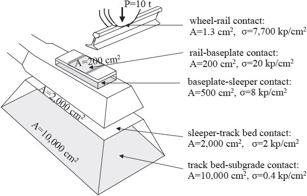
After Profillidis (2014), §7.2, Fig. 7.3. Full reference under Supplemental Sources.
| Parameter | Typical value |
|---|---|
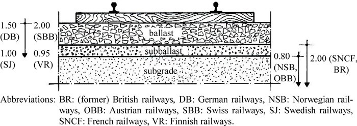
| Depth below ties | 12–18 in. (8 in. for yard and secondary track) |
| Shoulder width, tangent and inside of curves | 8–12 in. |
| Shoulder width, outside of curves | 12–18 in. |
| Shoulder slope | 2:1 to 3:1 (excess width or slope can block internal drainage) |
Stress under passing trains is about 6,000 psf just below the ties and falls to about 200 psf at 5 ft depth, before any dynamic allowance. At the rail, a loaded tank car’s weight spreads over about 19 ft (roughly 11 ties), and it continues to spread through the ballast and subgrade. A thin or degraded ballast and sub-ballast section concentrates stress into a smaller area of subgrade than the design assumed. The course states that substructure condition is the leading cause of track-geometry degradation, and that the substructure is what fails about 80% of the time when track has a problem.
Figures · click to zoom
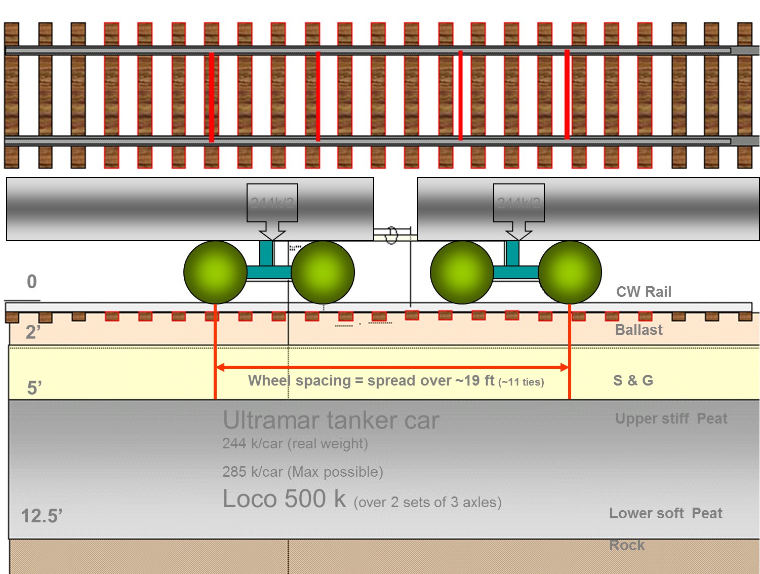
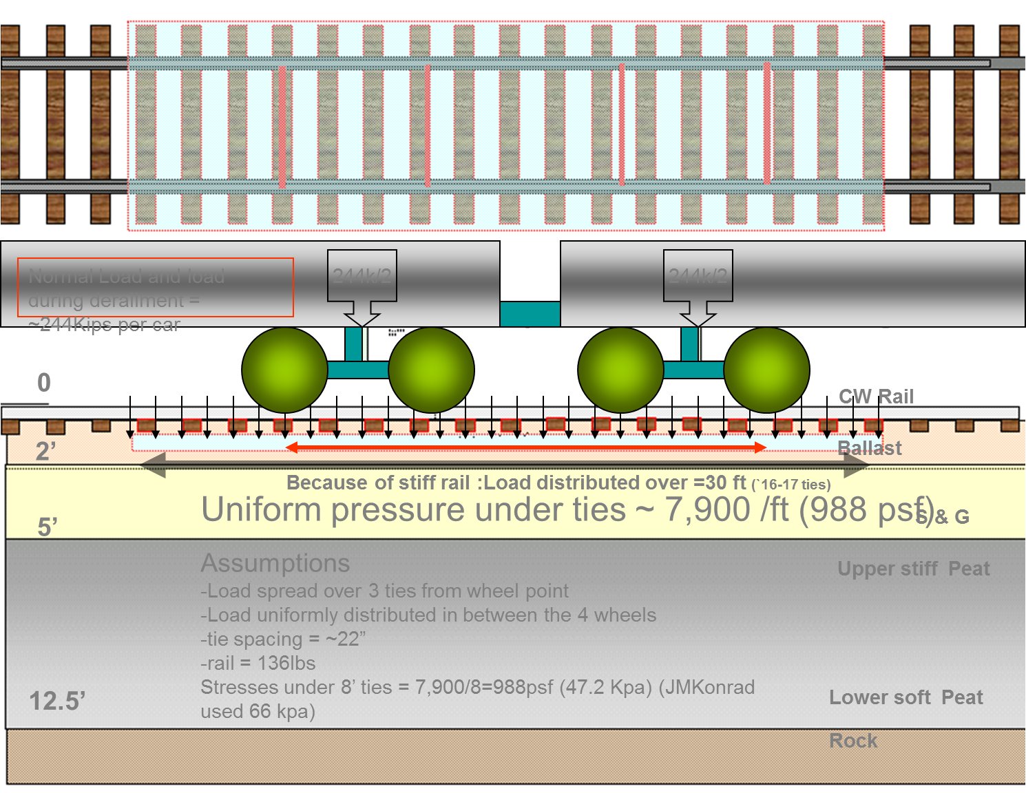
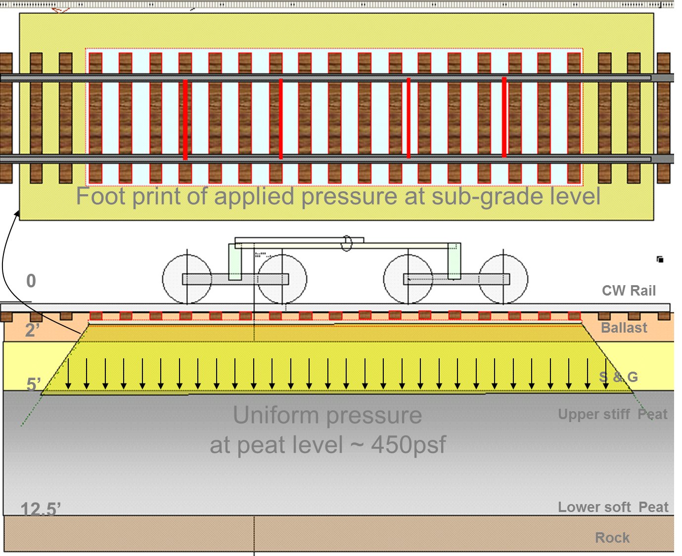
After Geotechnology for Railroaders Program, Module 3; §02–03, §13. Full reference under Supplemental Sources.
The Talbot (1920) equation distributes rail wheel load through the track structure to estimate contact pressure at the base of the tie (subgrade of the ballast):
p = P / (3 × L × U^(1/3)) [AREMA MRE Ch. 1, Sec. 1.3.5]
However, the more commonly used formulation for stress at the top of subgrade is the simplified Talbot distribution that treats the ballast and subballast as a combined bearing layer.
Reference graphics · click to zoom
The vertical stress at the top of subgrade beneath a single tie is estimated using the Talbot stress distribution:
σ_s = (P_d) / (A_eff) (psf)
where:
P_d = P_w × DLF (lb, dynamic wheel load)
A_eff = (B_t + 2 × d × tan θ) × (L_t + 2 × d × tan θ) (ft²)
For a single dynamic wheel load P_d = 40,000 × 1.3 = 52,000 lb and d = 2.0 ft (24 in. ballast + 12 in. subballast):
A_eff = (0.667 + 2 × 2.0 × 0.700) × (8.5 + 2 × 2.0 × 0.700)
= (0.667 + 2.80) × (8.5 + 2.80)
= 3.467 × 11.30 = 39.2 ft²
σ_s = 52,000 / 39.2 = 1,327 psf = 0.66 tsf
This is the design stress at the top of subgrade used for bearing capacity checks and to assess subgrade failure potential.
Selig and Waters ran a multilayer model study (GEOTRACK, 32,900-lb wheel) to see which design choices change rail seat load, ballast pressure and subgrade stress most. Use it to decide where design effort pays.
| Change | Effect |
|---|---|
| Tie spacing 10 → 36 in. | Rail seat load ×3; stress at ballast surface ×4; subgrade stress +50% |
| Rail moment of inertia 38.7 → 150 in.4 | Rail seat load −40% |
| Ballast depth 24 → 6 in. | Subgrade stress more than doubles: the strongest lever on subgrade stress |
| Ballast modulus 100,000 → 8,000 psi | Ballast strain ×9 |
| Tie stiffness | Stiff ties act as rigid footings and push peak ballast pressure to the tie ends; flexible ties peak under the rail seat. Subgrade stress is similar either way. |
Rail seat load is shared about 36% by the tie under the wheel, 22% by each adjacent tie and 10% by the next.
Quick hand checks.
Measured values for comparison. At FAST, wheel loads of 14,000 to 32,900 lb gave the following:
Ballast type (limestone, traprock or granite) had no detectable effect on the resilient response. These values are consistent with the roughly 10-psi subgrade stress in Table 2-1, which makes them a useful reasonableness check.
After Selig & Waters (1994), ch. 5. Full reference under Supplemental Sources.
| Ballast + Subballast Thickness (in.) | σ_s (psf) | σ_s (tsf) |
|---|---|---|
| 18 | 2,190 | 1.10 |
| 24 | 1,327 | 0.66 |
| 30 | 900 | 0.45 |
| 36 | 660 | 0.33 |
| 42 | 510 | 0.26 |
| 48 | 410 | 0.21 |
Subgrade bearing capacity is checked against σ_s. For soft fine-grained subgrades (CBR < 4), ballast and subballast thickness ≥ 36 in. is typically required to reduce stress to manageable levels.
AREMA allows several equations for stress at the top of subgrade:
Here Pm = 2 × rail seat load × impact factor ÷ effective tie bearing area. The effective area and the limit on Pm depend on tie type:
The traditional universal subgrade limit of 20 psi is too high for soft soils and too conservative for strong ones. Table 2-SW2 gives soil-specific values.
| Subgrade | psi |
|---|---|
| Compact till or hardpan | 65–100 |
| Gravel, very compact / loose | 55–85 / 25–50 |
| Coarse-to-medium sand, very compact / loose | 30–50 / 15–25 |
| Fine sand, loose | 8–15 |
| Clay, very stiff to hard | 25–50 |
| Clay, medium to stiff | 8–25 |
| Clay, soft | 4–8 |
| Silt, very stiff / soft | 15–30 / 4–8 |
These values come from static bearing practice and may still be unconservative under millions of load repetitions. For soft or wet fine-grained subgrade, check the granular depth with the threshold-stress approach in §2.4.2.
After Selig & Waters (1994), ch. 10. Full reference under Supplemental Sources.
The classical assumption is that the tie under a wheel carries 50% of the wheel load and each neighbor 25%. Stress measurements and finite-element analysis give a different split: 40% on the tie under the load, 23% on each adjacent tie and 7% on each second tie, with negligible effect beyond.
Track and wheel defects add a dynamic load, so analysis should use Qtot = Qstat + Qdyn, where Qdyn can reach 50% of the static wheel load. For a 11-ton wheel at 124 mph the measured increment was 4.4–6.6 tons. The book separates three frequency bands: 0.5–15 Hz (sprung mass, rolling-stock dependent), 20–100 Hz (unsprung mass, governed by track quality and stiffness) and 100–2,000 Hz (rail corrugation). Empirical dynamic impact factors close to measured values range from 1.35 to 1.6 at 125 mph, and 1.5 is suggested near that speed. Compare these with the AREMA impact allowance used in this section, which remains the design basis.
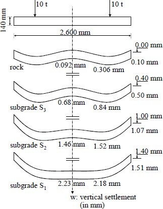
Elastoplastic finite-element runs (Figure 2-14) show that stress at the top of subgrade depends mainly on subgrade quality and only secondarily on track-bed thickness. With all else equal, moving the subgrade up one class (S1→S2, S2→S3, S3→rock) increases the stress developed in the subgrade by about 50%: a stiffer subgrade attracts more load, but carries it with far less settlement.
Figures · click to zoom
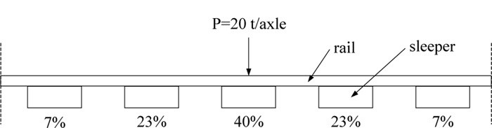
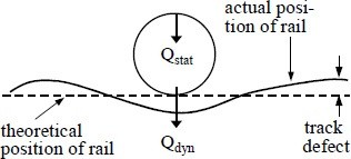
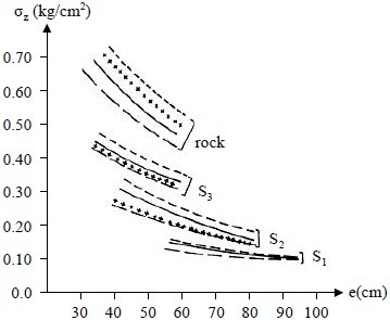
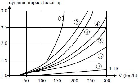
After Profillidis (2014), §7.11.2, §8.4.7–8.4.8, §8.6–8.7, Figs. 8.7, 8.10, 8.14, 8.15. Full reference under Supplemental Sources.
The track is a load-spreading system. It takes a concentrated wheel load at the rail head and spreads it along the track, across it and down through the section until the subgrade can carry it. Track that is well designed, built and maintained shares the load evenly, so each component carries its part. The designer’s job, on new track or on an upgrade of existing track, is to select a section that carries the design wheel load without overstressing any of the four main components: rail, ties, ballast and subgrade.
Along the track. When a wheel sits directly over a tie, that tie carries less than half of the wheel load. The rest goes to the two ties on each side (Figure 2-S5). For a 30,000-lb wheel on good track the UFC example split is 40% / 20% / 10%. That is close to the 40 / 23 / 7 finite-element split given above.
Down through the section. Pressure at the wheel–rail contact, about 60,000 psi over roughly ½ sq in., falls to about 300 psi on the tie plate, about 40 psi at the base of the tie and about 10 psi (1,440 psf) at the top of subgrade (Figure 2-S6). That is the same order as the Table 2-1 values for 18 to 24 in. of ballast and subballast, so it is a quick reasonableness check on a Talbot calculation. Actual pressures vary with wheel load, track section and track condition.
Figures · click to zoom
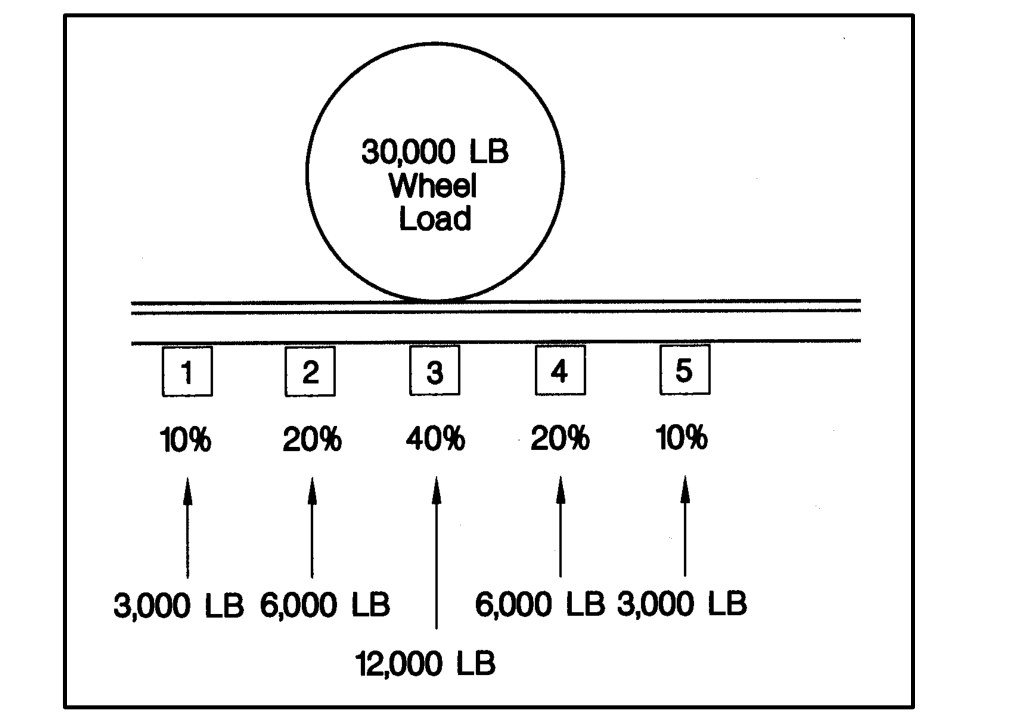
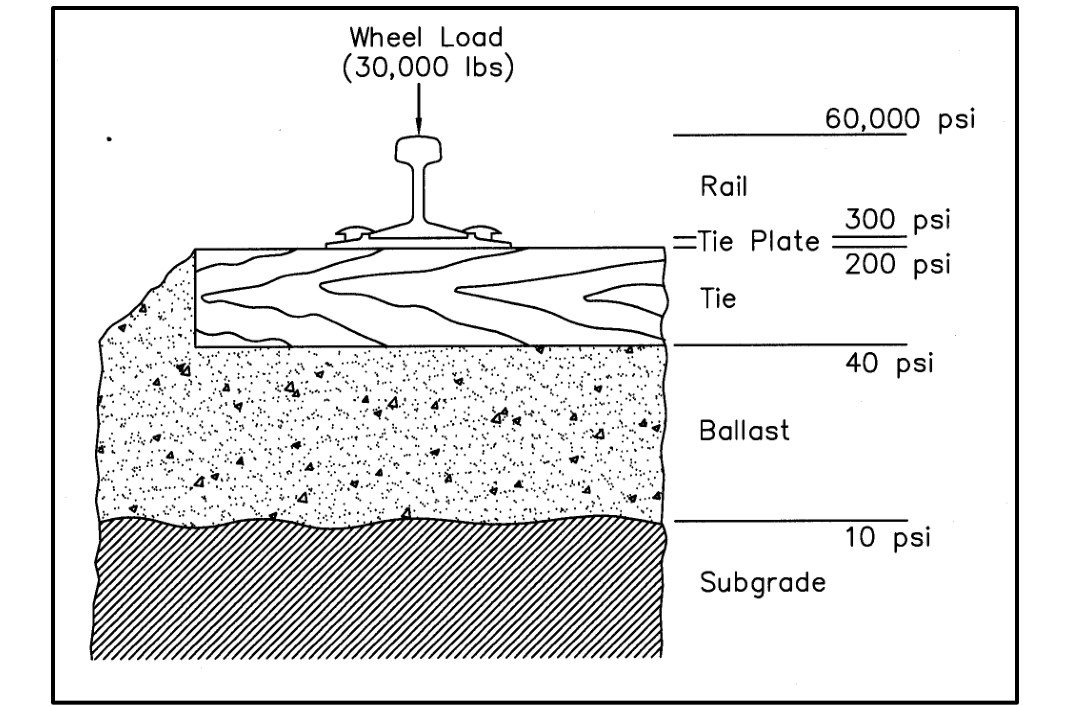
Design point. Track is simple to build, but its behavior under load is not. Strengthening one component can increase the load on another. When a rehabilitation changes one component (rail section, tie type or spacing, ballast depth), recheck the others, including the stress at top of subgrade in §2.2.1.
After UFC 4-860-01FA (2004), ch. 6, §5, Figs. 6-10 and 6-11. Comparison with §2.2 and Table 2-1 added by the authors. Full reference under Supplemental Sources.
Set the design wheel load from the heaviest loaded car that commonly runs over the track, not the rare heaviest movement. A locomotive usually puts down the heaviest single wheel. On most track, though, loaded-car wheels far outnumber locomotive wheels, so the car wheel load governs in most cases. Check both before the design is final.
The design wheel load is the static wheel load of that car plus an allowance for speed and for track and wheel irregularities. Table 2-S8 gives planning values for slow-speed track:
| Most common heavy car | 10–25 mph | ≤ 10 mph | Light use |
|---|---|---|---|
| Box, 40T | 20,000 | 17,600 | 16,000 |
| Box, 50T | 26,250 | 23,100 | 21,000 |
| Box, 70T | 34,375 | 30,250 | 27,500 |
| Flat, 40T | 17,500 | 15,400 | 14,000 |
| Flat, 50T | 23,750 | 20,900 | 19,000 |
| Flat, 80T (6-axle) | 23,750 | 20,900 | 19,000 |
| Flat, 100T (6-axle) | 32,500 | 28,600 | 26,000 |
| Flat, 140T (6-axle) | 38,750 | 34,100 | 31,000 |
| COFC, 70T | 30,000 | 26,400 | 24,000 |
| COFC, double stack | 50,000 | 44,000 | 40,000 |
| TOFC, 70T | 30,000 | 26,400 | 24,000 |
| Gondola, 40T high side | 18,750 | 16,500 | 15,000 |
| Gondola, 50T | 22,500 | 19,800 | 18,000 |
| Tank, 7,500 gal | 16,250 | 14,300 | 13,000 |
| Tank, 10,000 gal | 22,500 | 19,800 | 18,000 |
| Tank, 20,000 gal | 36,250 | 31,900 | 29,000 |
| Hopper, 50T | 21,250 | 18,700 | 17,000 |
| Hopper, 70T | 30,000 | 26,400 | 24,000 |
| Hopper, 100T (263K) | 41,125 | 36,190 | 32,900 |
| Hopper, 120T (286K) | 44,750 | 39,380 | 35,800 |
| Hopper, 125T (315K) | 49,250 | 43,340 | 39,400 |
| Locomotive, EMD GP7 / GP9 | 37,500 | 33,000 | 30,000 |
| Locomotive, EMD SW8 | 31,250 | 27,500 | 25,000 |
| Locomotive, 80-ton industrial | 25,000 | 22,000 | 20,000 |
| Locomotive, GE 65-ton | 20,000 | 17,600 | 16,000 |
| Locomotive, GE 40-ton | 13,750 | 12,100 | 11,000 |
Authors’ check: the Light use column equals the static wheel load (gross rail load ÷ 8 for a four-axle car; e.g., 286,000 ÷ 8 ≈ 35,800 lb). The ≤ 10 mph and 10–25 mph columns are the static value × 1.10 and × 1.25.
Limits on use. These speed allowances are lower than the 1.2 to 1.5 dynamic load factors used elsewhere in this manual because they assume slow operation. Use Table 2-S8 only for industrial, yard, terminal and light-density track. For mainline work, use Cooper E-80 or 286,000-lb loading with the client’s dynamic load factor (Part I, §I.4).
After UFC 4-860-01FA (2004), ch. 2, §4, Table 2-2. Car and locomotive designations as given in the source; factor check added by the authors. Full reference under Supplemental Sources.
How large the dynamic load is depends on the traffic. North American static wheel loads range from about 12,000 lb (light rail) to 39,000 lb (heavy haul). Measured dynamic loads compare as follows:
Rare heavy loads can control settlement. In box tests the order of loading did not change the final settlement. Once the largest load had been applied, smaller loads added almost nothing. A small share of heavy impacts, even 1 in 1,000, can therefore govern ballast settlement. Removing wheel flats, battered joints and rail defects is a substructure measure as well as a rail measure.
Uplift. The rail lifts the tie ahead of the wheel and then drives it back down. Where water is present, this pumps it.
Axle load and maintenance cost. German (DB) experience puts ballast maintenance cost roughly in proportion to the fourth power of ballast pressure, and British Rail concurs. By that rule, a 20% increase in axle load (for example, 100-ton to 125-ton cars) about doubles ballast maintenance. In box tests, raising the wheel load from 36 to 50 kips doubled the fines produced and tripled coarse breakage. DB responded with these changes:
Together they stretched tamping intervals from 1–2 years to 4–5 years. British Rail found lab settlement roughly proportional to axle load and to tie spacing. Going from 113 to 131 lb/yd rail (56 to 65 kg/m) cut settlement about 20%. Use these figures when a client asks what a heavier car fleet will cost in substructure maintenance (Chapter 1, §1.11).
After Selig & Waters (1994), chs. 2, 6 and 8. Full reference under Supplemental Sources.
AREMA MRE Chapter 1, Table 1-4.4-1 defines standard ballast gradations. The two most common for North American mainline freight service:
| Sieve Size | AREMA No. 4 (% Passing) | AREMA No. 24 (% Passing) |
|---|---|---|
| 2½ in. | 100 | 100 |
| 2 in. | 90–100 | 90–100 |
| 1½ in. | 25–60 | 60–90 |
| 1 in. | 0–10 | 10–35 |
| ¾ in. | 0–5 | 0–15 |
| ½ in. | — | 0–5 |
| No. 4 | 0–1 | 0–1 |
AREMA No. 4 is preferred for mainline heavy-axle freight (CSXT, NSR, UPRR, BNSF, CN). AREMA No. 24 (smaller size) is used by some clients (Amtrak, commuter rail) for improved ride quality and tamping.
Per AREMA Chapter 1, Section 1.4.4:
Client-specific ballast quality requirements:
| Railroad | LA Abrasion (max) | Soundness (max) | Preferred Rock Type | Governing Standard |
|---|---|---|---|---|
| CSXT | 30% | 5% Na₂SO₄ | Granite, limestone | CSXT Eng. Std. Sec. 6 |
| NSR | 30% | 5% Na₂SO₄ | Granite, quartzite | NSR Eng. Std. Manual Sec. 6 |
| G&W | 35% | 10% MgSO₄ | Local quarry approval | G&W Eng. Bulletin |
| UPRR | 30% | 5% Na₂SO₄ | Granite, basalt | UPRR Eng. Instr. Manual |
| BNSF | 30% | 5% Na₂SO₄ | Granite, limestone | BNSF Eng. Instructions |
| CPKC | 30% | 5% Na₂SO₄ | Granite (freeze-thaw) | CPKC Track Standards |
| Amtrak | 30% | 5% Na₂SO₄ | Granite preferred | Amtrak Eng. Std. |
| CN | 30% | 5% Na₂SO₄ | Granite (freeze-thaw) | CN Eng. Standards |
Reference graphics
Petrography first. A thin-section examination flags rock that will break down in track whatever the index tests say. Selig and Waters list these “fatal flaws” (after Watters et al.):
Abrasion tests measure different things.
In an AAR/Santa Fe test at about 300 MGT per year, fouling (minus No. 4) grew 0.4–0.6% per year, and 75–90% of it came from ballast breakdown. Fouling correlated with AN.
Shape. AREA adopted the Corps definitions in 1986: flat means thickness ÷ width < 1/3, and elongated means length ÷ width > 3, with a limit of 5% by weight. Flaky, angular particles raise shear strength, but they also break more, accumulate more permanent strain and lower stiffness.
Gradation. In laboratory tests, uniform ballast (Cu 1.14) showed about twice the plastic strain and 4–5 times the degradation of a broader gradation (Cu 4.1). The broader grading is stronger and settles less. But it has less void space to store fines, it can segregate, and it is more susceptible to fouling. CP ranks coarse uniform gradations best for fouling life, then fine uniform, then broad. The book finds no basis for a single optimum size. Durability and room to store fines govern.
Other indicators. Higher specific gravity goes with durability. Low absorption goes with weathering resistance. Higher rodded unit weight goes with lateral stability. Where limestone or other soft stone sits in wet track, a wet attrition (Deval) test is worth requesting. British Rail limited it to 4%.
After Selig & Waters (1994), chs. 3, 7 and 8. Full reference under Supplemental Sources.
Section 2.3.2 gives the AREMA limits. Li et al. (2016) add two screens that are worth requesting when qualifying a new quarry: the Mill Abrasion test (Selig & Waters, 1994), which wears the stone in water and is more sensitive than LA Abrasion to the soft, clay-bearing rocks that turn to mud in track, and petrographic analysis of the parent rock. Canadian Pacific’s limits show how far a freeze–thaw railroad tightens the AREMA values:
Table 2-S2. AREMA vs. Canadian Pacific ballast limits (Li et al., 2016, Table 3.3)
| Test | Procedure | AREMA | CPR |
|---|---|---|---|
| Los Angeles Abrasion | ASTM C535 | 35% max. | 45% max. (paired with Mill Abrasion) |
| Mill Abrasion | Selig & Waters (1994) | – | 9% max. |
| Absorption | ASTM C127 | 1.0% max. | 0.5% max. |
| Sulfate soundness | ASTM C88 | 5.0% max. | 1.0% max. (mainline) |
Table 2-S3. Rock properties that lead to poor ballast performance (after Watters et al., 1987)
| Rock property | Deterioration problem |
|---|---|
| Soft minerals (e.g., clay shale) | Rapid wear and crushing |
| Minerals that weather or deteriorate rapidly | Weathering of the stone in track |
| Poorly consolidated texture | Rapid abrasion |
| High porosity | Freeze–thaw deterioration |
| Smooth particle surface | Poor stability |
| Long, flat particle shape | Poor stability; breakage of elongated pieces |
Li et al. recommend petrographic analysis of the parent rock whenever a new source is being qualified, because it shows secondary minerals and textures that the index tests can miss.
Source: Li, D., Hyslip, J., Sussmann, T. and Chrismer, S. (2016). Railway Geotechnics. CRC Press / Taylor & Francis
The European standard designates ballast by a pair of sieve sizes, 1¼ in. lower and 2 in. or 2½ in. upper, and lets the supplier declare a category for each property. The Los Angeles test is the reference hardness test (in the EN version: 22-lb sample, 1,000 revolutions at 31–33 rpm). Many older regulations simply require LA < 25.
| Los Angeles coefficient | Category | Micro-Deval coefficient | Category |
|---|---|---|---|
| ≤ 12 | LARB12 | ≤ 5 | MDERB5 |
| ≤ 14 | LARB14 | ≤ 7 | MDERB7 |
| ≤ 16 | LARB16 | ≤ 11 | MDERB11 |
| ≤ 20 | LARB20 | ≤ 15 | MDERB15 |
| ≤ 24 | LARB24 | > 15 | declared |
| > 24 | declared |
| Property | Category limits |
|---|---|
| Fine particles (passing No. 35) | A: 0.6% · B: 1.0% · declared > 1.0% |
| Fines (passing No. 230) | A: 0.5% · B: 1.0% · C: 1.5% · declared > 1.5% |
| Flakiness index | ≤ 15, ≤ 20, ≤ 35, declared > 35 |
| Shape index | ≤ 10, ≤ 20, ≤ 30, 5–35, declared > 30 |
| Particles ≥ 4 in. long (sample > 88 lb) | A: 4% · B: 6% · C: 8% · D: 12% |
Deval requirements in older regulations range from a coefficient greater than 12 (limestone) or 14 (hard rock) to greater than 16, which may exclude limestone and push a railway toward granite. French practice requires the LA and Deval results to plot together inside an acceptance band (Figure 2-18).
Figures · click to zoom
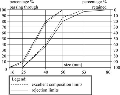
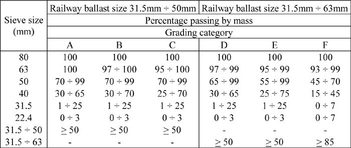
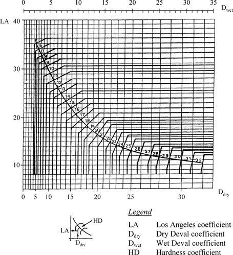
After Profillidis (2014), §12.2–12.4, Tables 12.2–12.9, Figs. 12.1, 12.5; after EN 13450 (2002). Full reference under Supplemental Sources.
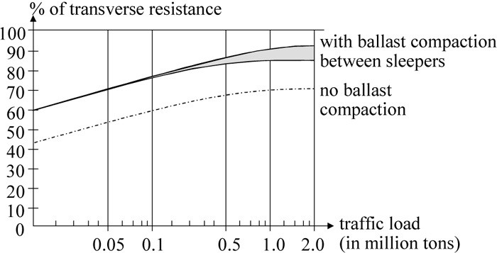
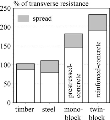
Lateral (transverse) track resistance has three parts: friction under the tie (proportional to tie weight), friction along the tie sides from crib ballast, and passive resistance at the tie ends from the shoulder. The crib component is about 40–50% of the total for timber ties, 30% for monoblock concrete and 15–25% for twin-block ties, so under-filled cribs cost timber track the most.
These numbers explain why slow orders follow surfacing and undercutting, and why shoulder width and crib fill should be checked wherever a ground-hazard repair has disturbed the ballast section.
Figures · click to zoom
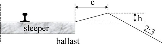
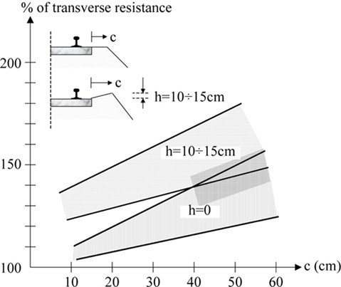
After Profillidis (2014), §13.3–13.6, Figs. 13.2, 13.3, 13.6, 13.7. Full reference under Supplemental Sources.
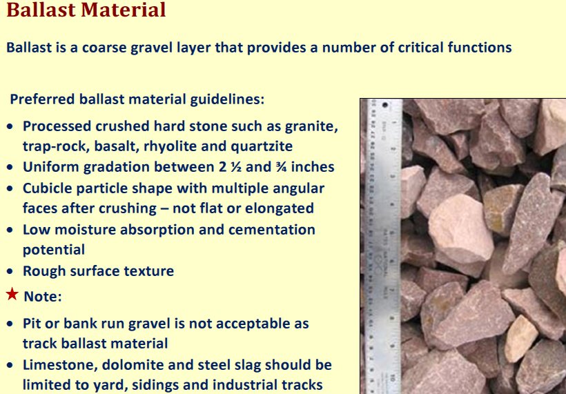
Ballast does six jobs: drainage, load distribution, vertical stiffness, longitudinal hold, lateral hold, and making surfacing practical. Failure of a function shows in the geometry: 2.5 in. or more of rail deflection at a joint means load distribution has failed, uneven support shows as cross-level, and ballast plowed in the direction of travel means it is too fine to hold the track. Judge ballast by digging, not by the surface.
Ballast shear strength comes from friction, which depends on size, angularity and interlocking. Prefer hard, dark, fine-grained extrusive rock (andesite, basalt, micro-diorite). Limestone, quartz, metamorphic rock and shale are unsuitable, and soft rock can grind into a mud spot within 2–3 years. Ballast life is roughly 200–900 MGT depending on rock type: some limestone lasts about 300 MGT, andesite about 900 MGT.
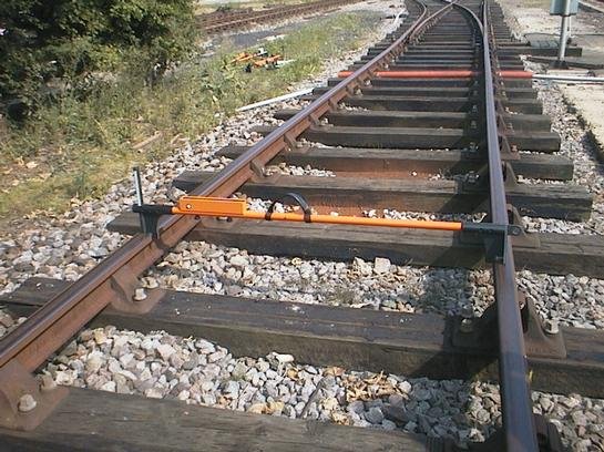
Shoulder width is a standard to enforce, not tolerate. A minimum 12-in. shoulder is what holds the ties laterally, and inadequate shoulders can contribute to derailments.
Figures · click to zoom
After Geotechnology for Railroaders Program, Module 3, Module 2; Module 3 §04–05, §11; after Selig & Waters (1994). Full reference under Supplemental Sources.
Seeley’s chapter on measuring rail track (CESMM3 Class S) sets out conventions that carry over to North American work:
His example is 492 ft of straight single track with ballast 10.33 ft wide, a 6-in. bottom ballast layer and about 5 in. of top ballast, timber ties at 29.5-in. centers, and 113 lb/yd rail.
Table 2-PM1. Table: Take-off for 492 ft of single track (after Seeley 1993, Example XVIII, converted to US units)
| Item | Calculation | Quantity |
|---|---|---|
| Bottom ballast | 492 × 10.33 × 0.49 ft | 92.7 CY |
| Top ballast (no deduction for ties) | 492 × 10.33 × 0.43 ft | 80.3 CY |
| Ties | 492 ft / 2.46 ft + 1 | 201 each |
| Rail, supply only | 2 rails × 492 ft at 113 lb/yd | 18.5 tons |
| Track laying | centerline length | 492 ft |
For railroad work: when a geotechnical design calls for undercutting and new subballast and ballast, give the quantities in the same structure that the track contractor and the railroad’s material desk use. List separately:
State whether the ballast volume deducts the ties, and convert to tons with a unit weight measured for the actual quarry source. That way the engineer’s tonnage and the tonnage the railroad orders are computed on the same basis.
Source: Seeley, I. H. (1993). Civil Engineering Quantities, 5th ed. Basingstoke: The Macmillan Press, pp. 237–241. Summarized and paraphrased. Full reference under Supplemental Sources.
Subballast serves as a transition filter between ballast and subgrade, provides drainage, and distributes load. AREMA Chapter 1, Section 1.4.5 specifies:
| Sieve | % Passing |
|---|---|
| 1½ in. | 100 |
| ¾ in. | 55–85 |
| No. 4 | 30–60 |
| No. 10 | 20–50 |
| No. 40 | 10–25 |
| No. 200 | 0–7 |
Filter compatibility between subballast and subgrade must be verified using Terzaghi filter criteria:
D₁₅(subballast) / D₈₅(subgrade) < 5 (piping criterion)
D₁₅(subballast) / D₁₅(subgrade) > 5 (permeability criterion, for drainage)
Reference graphics
Material. Selig and Waters base North American subballast requirements on ASTM D1241:
Under saturated repeated loading, crushed rock with no plastic fines performed best and natural rounded gravel performed worst.
Filter criteria. The subballast must satisfy these against the subgrade below and against the ballast above:
For medium- to high-plasticity clay with no silt or sand, D15 of the filter may be up to 0.016 in., provided Cu ≤ 20 to limit segregation. Confirm with a repeated-load filter test, because the criteria were developed for steady seepage.
Permeability balance. Subballast should be at least 10 times less permeable than the ballast, with a sloped surface, so that rain sheds sideways instead of soaking the subgrade. It still needs to be more permeable than the subgrade so upward seepage can escape. In frost areas, do not add fines to lower the permeability.
When one gradation will not work. A single layer between AREMA No. 4 ballast and a fine subgrade would have to span fine gravel to silt. In that case, use two layers. The upper, coarser layer is matched to the ballast. The lower layer is a blanketing sand matched to the subgrade (Table 2-SW3).
| Sieve | % passing |
|---|---|
| ½ in. | 100 |
| No. 8 | 80–100 |
| No. 16 | 70–90 |
| No. 30 | 48–76 |
| No. 50 | 24–60 |
| No. 100 | 5–42 |
| No. 200 | 0–10 |
Frost. Where frost and water can reach the subballast, keep silt plus clay below about 5%.
Placement. Shape and compact the subgrade to drain before placing subballast. Then:
After Selig & Waters (1994), ch. 9. Full reference under Supplemental Sources.
Where native subgrade is soft (CBR < 3) or frost-susceptible, a blanket layer of select granular material is required between the subgrade and subballast. This is often called a "capping layer" or "sub-base" in international railroad practice.
Minimum blanket thickness to reduce σ_s to acceptable level:
From Table 2-1, select d (ballast + subballast + blanket total) to achieve σ_s ≤ σ_allow(subgrade).
For soft clay subgrade with q_u = 1,200 psf, AREMA recommends:
σ_allow = q_u / (π + 2) × FS where FS ≥ 3.0 for cyclic loading
σ_allow = 1,200 / (5.14 × 3.0) = 78 psf
This requires d ≥ 54 in. from Table 2-1, or supplemental ground improvement (see Chapter 17).
Typical minimums. North American practice has used the following:
These values set ballast depth for tamping, fines storage and filtering. They do not, by themselves, protect a weak subgrade. Size the combined ballast and subballast (the “granular layer”) separately, to prevent progressive shear and excessive cumulative plastic settlement.
Threshold stress. Repeated-load triaxial tests show a cyclic deviator stress that separates two behaviors:
The threshold rises roughly linearly with confining stress. British Rail sets the granular depth where the traffic-induced stress drops to the threshold stress. For example, a 16-tonne (35-kip) axle on a subgrade with a 8.7-psi threshold needs about 24 in..
British Rail practice.
Field validation. Subgrade movement (mm per million axles) was rapid where the actual granular depth was less than the design depth and slow where it was greater. Deepening the ballast stabilized a previously unstable site.
This method complements the Li–Selig method above. Use the threshold check as a quick screen, and use Li–Selig where the design tonnage and cumulative deformation must be shown explicitly.
After Selig & Waters (1994), ch. 10. Full reference under Supplemental Sources.
The Talbot-type equation in AREMA (H = 0.24 (Pm/Pc)0.8, with a universal allowable subgrade stress of 20 psi) dates from field tests in the 1910s–1920s. Li et al. note it ignores subgrade type, repeated loading and material quality, so it is unconservative on soft soils and overly conservative on good ones. They compare four methods:
Table 2-S7. Comparison of granular layer design methods (Li et al., 2016, Table 5.1)
| Feature | AREMA equations | Raymond | British Rail | Li–Selig |
|---|---|---|---|---|
| Traffic | Single wheel | Single wheel | Single wheel | Multiple wheel loads and total tonnage |
| Subgrade property | None | Soil type | Threshold strength | Resilient modulus and compressive strength |
| Ballast property | None | None | None | Resilient modulus |
| Design criteria | 20 psi allowable | Allowable stress by soil class | Progressive shear | Progressive shear and cumulative deformation |
| Stress model | Empirical | Homogeneous | Homogeneous | Multilayer |
For heavy-haul mainline work on soft subgrade, the Li–Selig method (which checks both progressive shear and cumulative plastic deformation over the design tonnage) is the most defensible of the four; the Talbot result can be shown alongside it for comparison with client standards.
Source: Li, D., Hyslip, J., Sussmann, T. and Chrismer, S. (2016). Railway Geotechnics. CRC Press / Taylor & Francis
UIC Code 719R classes the subgrade by its expected behavior: S3 good (low settlement, very good support), S2 medium, S1 poor (large settlement), and S0 very poor, plus R for sound rock, which later UIC editions fold into S3. The class follows from fines content, plasticity, Los Angeles value for rock, and whether hydrogeological conditions are good or bad.
| Soil or rock description | Hydrogeological conditions | Subgrade class |
|---|---|---|
| Rock of very good quality | – | R |
| Well-graded soils with < 5% fines; hard rock with LA < 30 | – | S3 |
| Soils with 5–15% fines; sand with < 5% fines; moderately hard rock (30 < LA < 40) | good / bad | S3 / S2 |
| Soils with 15–40% fines; rock moderately susceptible to weathering; soft rock (LA > 40); silty sand and schist with PI > 7 | good / bad | S2 / S1 |
| Rock very susceptible to weathering; soils with > 40% fines; slightly plastic silt | – | S1 |
| Organic soils; soils with > 15% fines at high moisture; soluble soils (rock salt, gypsum); thixotropic soils (quick clay); mixed material / organic; contaminated ground | – | S0 |
Fines = particles smaller than 60 µm. Some railways place the mixed/organic soils in S1.
S0 soils settle heavily, are inhomogeneous, change with time and let ballast punch in. Avoid them in alignment where possible or replace them; where neither is possible, especially under high embankments, combine ground improvement with thicker ballast and subballast and a geotextile.
On S1 and S2 subsoil, UIC practice adds a formation layer of better material compacted to 100% Standard Proctor, against the 95% usually specified for embankment subsoil. It only works if the subsoil has a low water content (otherwise fines migrate up and spoil the crossfall) and the layer is homogeneous, without pockets of fine material.
| Subsoil class | Formation layer quality | Thickness (in.) |
|---|---|---|
| S1 | S2 | 12–22 |
| S1 | S3 | 8–16 |
| S2 | S3 | 8–12 |
Figures · click to zoom
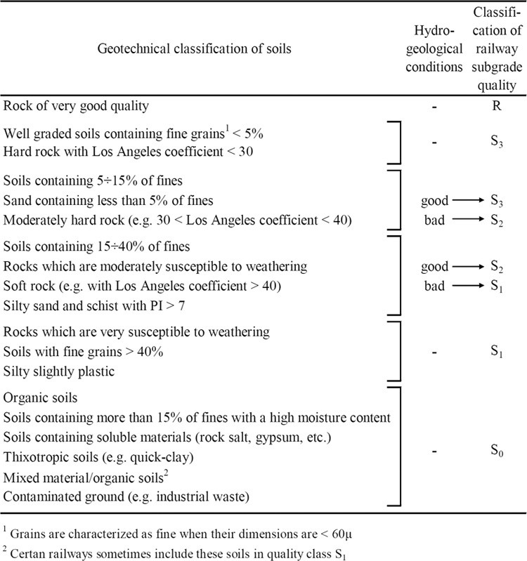
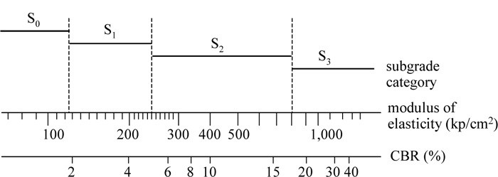
After Profillidis (2014), §9.5–9.7, Tables 9.2–9.3, Fig. 9.5; after UIC Code 719R (1994). Full reference under Supplemental Sources.
UIC sizes the total track bed (ballast + subballast) by adding corrections to a base value for subgrade class. The formula comes from the finite-element stress results in Figure 2-14:
| Term | Depends on | Values (in.) |
|---|---|---|
| N | Subgrade class | S1: 27.6 · S2: 21.7 · S3: 17.7 |
| a | UIC group | Groups 1–2 or V > 99 mph: 0 · 3–4: −2.0 · 5: −3.9 · 6: −5.9 |
| b | Tie type and length L | Timber (8.5 ft): 0 · concrete: (98.4 − L)/2, with tie length L in inches |
| c | Maintenance volume | Medium: 0 · high, groups 1–5: −3.9 · high, group 6: −2.0 |
| d | Axle load | 22 tons: 0 · 25 tons: +2.0 · 28 tons: +4.7 · 33 tons: +9.8 |
| f | Speed | V < 99 mph: 0 · high speed on S3: 0, on S2: +2.0, on S1: +3.9 |
| g | Geotextile | Geotextile thickness, or 0 if none |
Book example. UIC group 4 line, 8.5-ft monoblock concrete ties, S2 subgrade, 22-ton axles, medium maintenance, 124 mph, 0.2-in. geotextile: e = 21.7 − 2.0 − 2.0 + 0 + 0 + 2.0 + 0.2 = 19.9 in. (about 20 in.). With the usual 6-in. subballast, the ballast is 14 in., close to the 15 in. that British practice would give. The same site with a frost index of 540 °F-days needs 31 in. of track bed for frost protection (Figure 2-29), and the larger value governs.
North American check. A 286k car on 4 axles is about 35.7 tons/axle, beyond the formula’s 33-ton calibration point (d = +9.8 in.). Treat the formula as a cross-check on the AREMA/Talbot thickness in this chapter, not as a substitute.
UIC subballast is usually 6 in. of well-graded gravel with Micro-Deval < 15–20 and LA < 20–25 depending on the line’s importance; some railways require at least 30% crushed stone on new lines. Some railways omit subballast and use a thicker formation layer instead.
After Profillidis (2014), §12.1.2, §12.5.1–12.5.5, Eq. 12.8. Full reference under Supplemental Sources.
Sub ballast is a compacted, well-graded sand–gravel layer 6–12 in. thick between ballast and subgrade. It is often missing on century-old mainline. It drains as part of the lateral path, adds vertical strength, and separates ballast from fine-grained subgrade in both directions. Course specification: crushed or screened pit-run gravel graded 0–3 in. or 0–¾ in., less than 8% fines, no organics, well graded, and ideally at least 50% fractured faces. Watch for contractors offering fill with more fines than specified: it compacts well dry but performs poorly once wet.
Figures · click to zoom
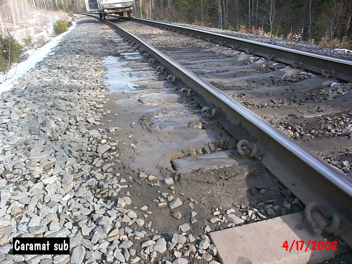
After Geotechnology for Railroaders Program, Module 3, Module 2; Module 3 §08; Module 2 §09. Full reference under Supplemental Sources.
Case study: 2.18.1 Zoning the best subgrade material, and losing it in the stockpile (Look 2023), in §2.18 Case Studies.
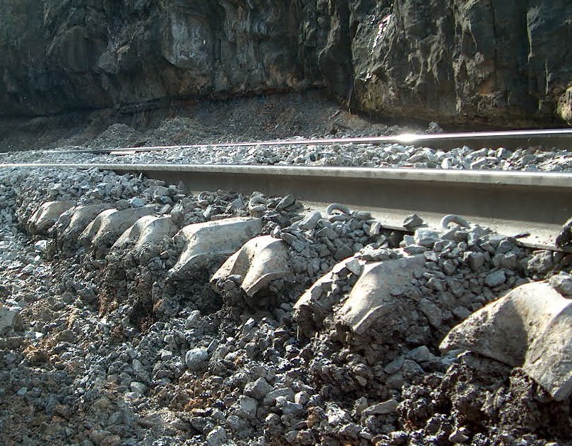
Progressive shear occurs when σ_s exceeds the undrained shear strength of the subgrade, typically in saturated fine-grained soils under repeated loading. Manifests as pumping, subgrade mud, and progressive track settlement.
FS against progressive shear:
FS_shear = (π + 2) × s_u / (DLF × σ_s_static) ≥ 3.0 (AREMA Ch. 1 recommendation for cyclic loading)
where s_u = undrained shear strength of subgrade (psf); σ_s_static = static stress at top of subgrade (psf).
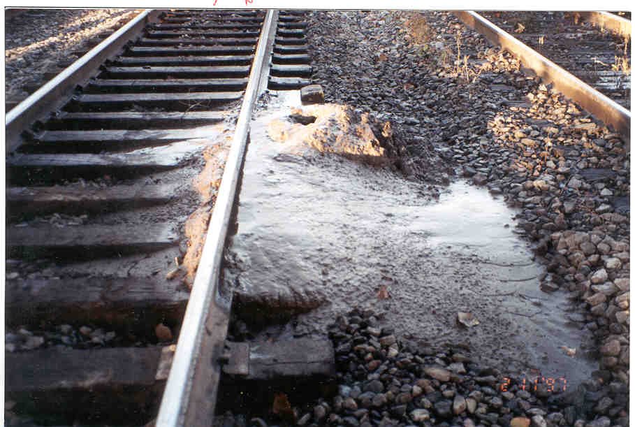
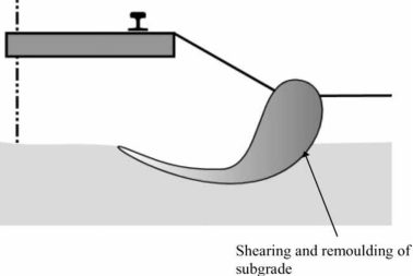
Mechanism. Repeated overstress at the top of a soft, fine-grained subgrade remolds the soil and squeezes it sideways and upward beside the track. It heaves the cess (the area beside the track) and leaves a depression under the ties. The heave then walls off the side drainage, raises the water table under the track and speeds up the failure. Segmented tubing columns installed through the shoulder show whether the heave is still active.
Massive shear needs much higher stress than progressive failure. It usually happens when strength drops because of water, such as heavy rain or flooding, sometimes with no train present.
What does not work.
Repair. Remove the ballast and excavate the failed subgrade to a lower, regular surface sloped to drain. Rebuild with subballast or blanket and clean ballast to the depth from §2.4.2, and restore the side drainage. The two preventive measures are adequate granular depth and drainage that keeps the water table low.
After Selig & Waters (1994), ch. 10. Full reference under Supplemental Sources.
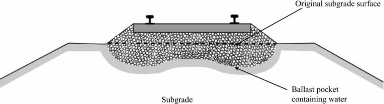
Ballast pockets form when fine-grained subgrade material is pumped upward through ballast voids under dynamic loading. Indicators:
Prevention: Properly designed subballast filter layer; maintain drainage; GPR monitoring.
Ice lens formation in frost-susceptible subgrade causes differential heave across a cross-section or along the track. NSR, CPKC, and CN experience significant frost heave problems.
Differential heave threshold: FRA 49 CFR Part 213 Class 4 surface tolerance = 1.25 in. over 62 ft chord.
Design mitigation:
Frost heave needs freezing temperatures, a supply of water and a frost-susceptible soil, all at once. Remove any one and heave stops. Ice lenses can heave the ground by much more than the roughly 10% volume increase of freezing water alone. On thaw, the released water softens the subgrade and geometry is lost quickly.
How susceptible the soil is depends on its type:
Ballast and subballast insulate the subgrade, and the required thickness is usually set by local experience. Where frost and water reach the subballast, keep its fines below about 5%. On a frost-susceptible embankment over a shallow water table, a geomembrane placed above the water table and below the maximum frost depth can cut off capillary supply (Chapter 17, §17.8.1).
After Selig & Waters (1994), chs. 9 and 12. Full reference under Supplemental Sources.
Repeated cyclic loading degrades the subgrade surface through abrasion, generating fines that contaminate ballast. Most common in granular subgrades under high-axle-load traffic. Prevent with properly graded subballast and geotextile separator.
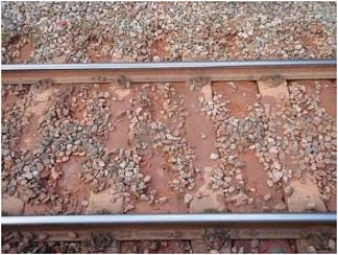
Where it occurs. Selig and Waters tie subgrade attrition to ballast bearing on hard fine-grained soil (stiff clay) or soft rock (chalk, mudstone, shale) with standing water at the subgrade surface. The ballast grinds the surface into a slurry, and traffic pumps the slurry up to the tie, often at rail joints. The slurry then blocks the drains. This is a narrower setting than the general description above, and it matters when choosing the remedy.
Look-alikes. Ballast and tie wear in wet conditions, and plain dirty ballast, also produce mud at the surface. Before choosing a fix, compare the fines in the slurry with the subgrade, checking plasticity, color and mineralogy.
What fixes it. Two measures together:
Ballast cleaning alone gives only temporary relief. British Rail made attrition failures rare by blanketing.
The record on geotextiles.
Design point: a sand blanket stops clay pumping, and fabric alone does not.
After Selig & Waters (1994), chs. 10 and 12. Full reference under Supplemental Sources.
Sections 2.5.1–2.5.4 cover four subgrade problems; Li et al. recognize ten. Li et al. group them by what drives them — dead load, live (train) load, or the environment — which is a useful way to tie field symptoms back to a cause before selecting a remedy.
Table 2-S6. Characteristics of track subgrade problems (Li et al., 2016, Table 3.9)
| Cause | Type | Contributing factors | Field features |
|---|---|---|---|
| Dead load | Massive shear failure | Weight of train, track and subgrade; inadequate soil strength | High embankments and cut slopes; often triggered by a rise in water content |
| Dead load | Consolidation settlement | Embankment weight; saturated fine-grained soils | Increased static stress vs. pre-construction |
| Live load | Subgrade attrition | Ballast bearing directly on hard subgrade; clay-rich rock or soil; water | Muddy ballast; missing or inadequate subballast |
| Live load | Cyclic mobility / liquefaction | Repeated loading of saturated silt and fine sand | Large displacement; worse with vibration; can occur in subballast |
| Live load | Progressive shear failure | Repeated overstressing of wet fine-grained soil | Squeezing at subgrade surface; heave in crib or shoulder; depression under ties |
| Live load | Cumulative plastic deformation | Repeated loading of soft or loose soil | Differential settlement; ballast pockets |
| Environment | Frost action | Freezing temperatures, free water, frost-susceptible soil | Rough surface in winter/spring |
| Environment | Swelling / shrinkage | High-plasticity soil with changing moisture | Rough track surface |
| Environment | Slope erosion | Surface and subsurface water; wind | Soil washed or blown away |
| Environment | Soil collapse | Water inundation of loose deposits | Ground settlement |
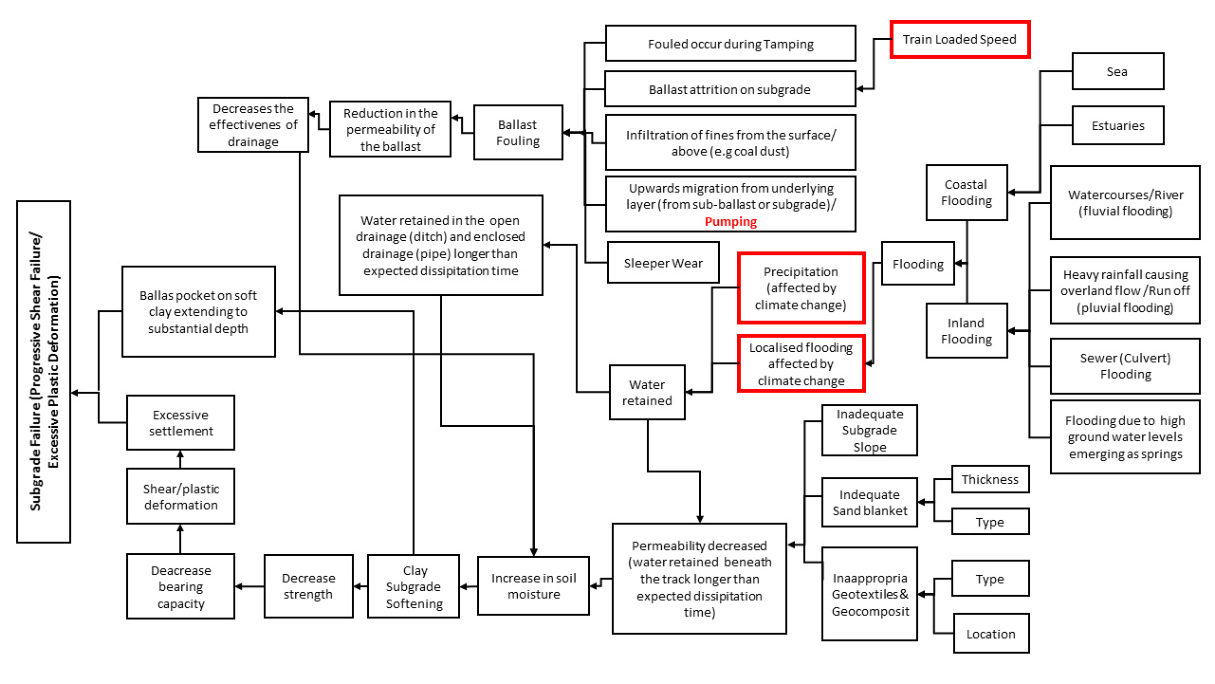
Usman et al. (2015) add a drainage-focused view: most live-load failures on fine-grained subgrade start with water retained in the track section (fouled ballast, blocked ditches, clogged pipe drains), which softens the clay, lowers its strength and bearing capacity, and leads to shear/plastic deformation and ballast pockets. Their cause-and-effect chart (Figure 2-S4) is a practical checklist for tracing a wet spot back to the drainage element that failed. UK surveys cited in the paper found an average of about five wet spots per mile of track.
Source: Li, D., Hyslip, J., Sussmann, T. and Chrismer, S. (2016). Railway Geotechnics. CRC Press / Taylor & Francis · Usman, K., Burrow, M. and Ghataora, G. (2015). “Railway track subgrade failure mechanisms using a fault chart approach.” Procedia Engineering 125, 547–555 (open access, CC BY-NC-ND 4.0)
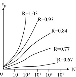
For soils, fatigue shows up as accumulating plastic strain rather than sudden fracture. Repeated-load triaxial tests on clays (Figure 2-25) use R, the ratio of the first-cycle deviator stress to the deviator stress that causes failure. Above R ≈ 0.9, plastic strain increases very rapidly with the number of cycles. Below it, strain grows roughly with log N and levels off. The runaway behavior was observed in S0 and S1 subgrades.
For the effect of traffic on subgrade stress the book uses Dormon’s rule from highway practice: σ1/σ2 = (N2/N1)λ, with λ ≈ 0.2. For two lines with the same axle load, the allowable subgrade stress therefore scales with (T2/T1)0.2: doubling tonnage lowers the allowable stress by about 13%.
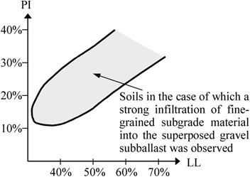
Subgrade fines can also migrate upward. Figure 2-26 shows the combinations of plasticity index and liquid limit for which strong infiltration of subgrade fines into a gravel subballast was observed. It is a useful screen when deciding whether a separation geotextile or sand blanket is needed.
Figures · click to zoom
After Profillidis (2014), §9.8, §9.10, §9.15.2, Figs. 9.7, 9.19. Full reference under Supplemental Sources.
The frost index is the time integral of below-freezing temperature (°F × hours or °F × days). A railway must choose whether to design for the coldest winter or for an average winter and accept occasional frost penetration. Silt is very frost-susceptible, clay is susceptible, and sand and gravel are not.
| Frost index | Probability of freezing through | Expected number of underratings |
|---|---|---|
| F2 | 50% | 1 in a 2-year period |
| F5 | 20% | 1 in a 5-year period |
| F10 | 10% | 1 in a 10-year period |
| F100 | 1% | 1 in a 100-year period |
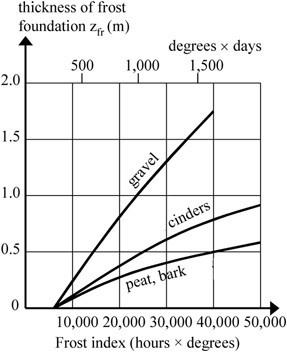
The required frost-protection layer under 14 in. of ballast increases with frost index and depends on the material (gravel needs the most, peat/bark the least; Figure 2-27). A foam-plastic insulation board 2–4 in. thick sharply reduces the required thickness (Figure 2-28). On existing track, frost protection is normally installed at renewal using one of four details: a gravel or cinder layer, stone with a peat filter, foam plastic, or insulation over a frost-storage bottom layer.
Figures · click to zoom
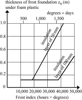
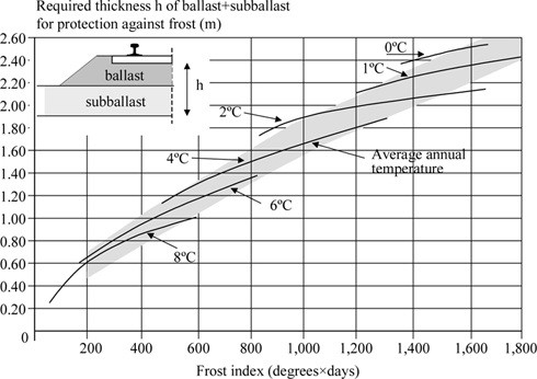
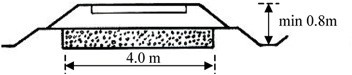
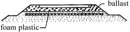
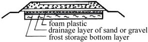
After Profillidis (2014), §9.11, §12.5.2, Table 9.6, Figs. 9.8–9.13, 12.6. Full reference under Supplemental Sources.
Before touching a mud spot, ask what kind it is and how deep the problem goes. The cause is usually ballast degradation, subgrade liquefaction and pumping, plastic deformation, subgrade failure, or poor drainage. The fix ranges from tamping (temporary) to undercutting or reinforcing the subgrade (durable). One railroad spent nearly $10M in a year on mud spots and wasted about 90% of it treating symptoms. On another system, over 95% of a $200M+/year ballast budget went into the upper 20 in. of the structure.
On a steep embankment, uncorrected ballast pockets can become a slope failure. In one silt-pumping case, an investigation trench beside sinking track showed silt rising as the track went down. The fix was filter cloth, gravel backfill and deeper ditches, which addressed the water path rather than the sinking.
Figures · click to zoom
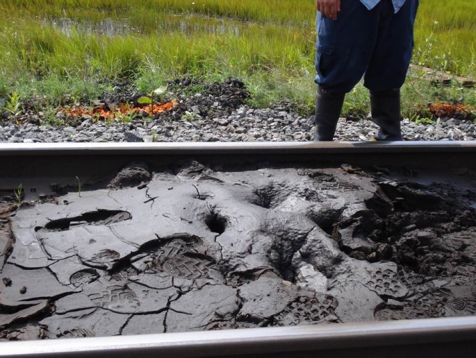
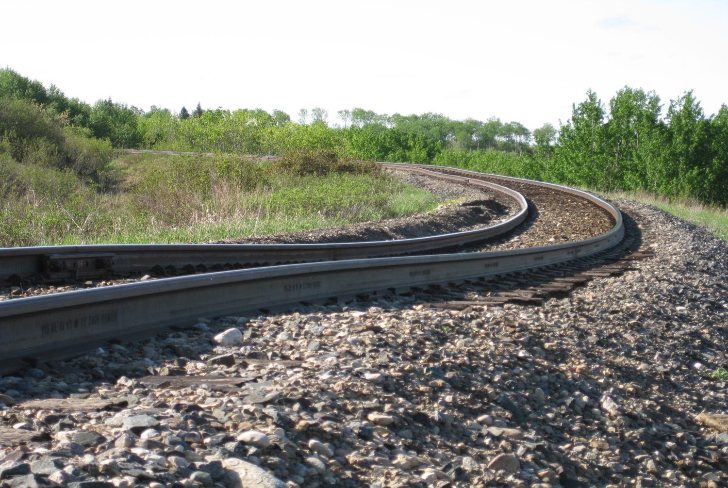
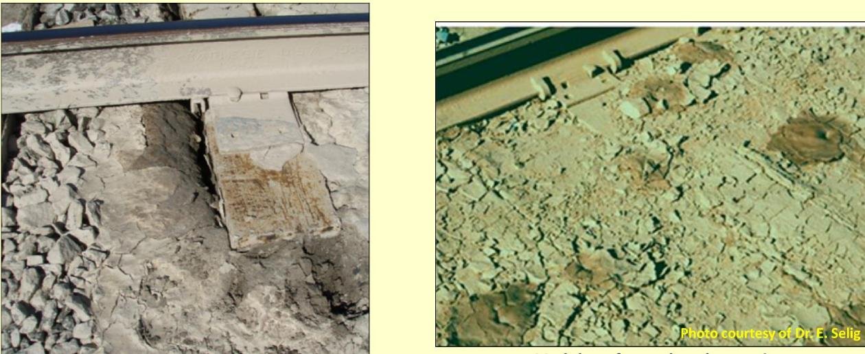
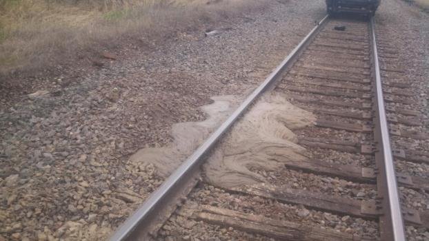
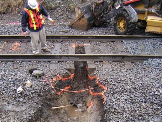
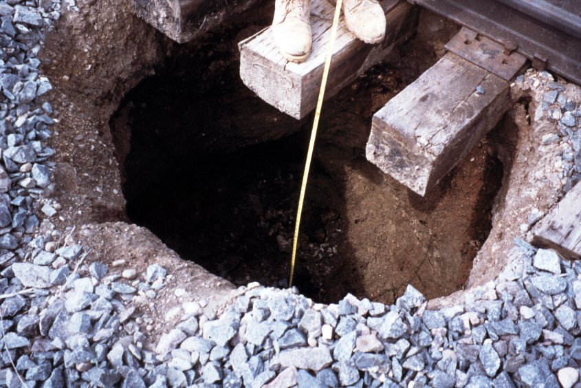
After Geotechnology for Railroaders Program, Module 3; §02, §09, §11. Full reference under Supplemental Sources.
Frost heave needs five conditions at once: saturated soil, frost-susceptible soil (silt), sub-zero temperature, a slowly advancing freezing front, and a water supply from below. Remove any one and it cannot occur. About 75% of heave problems trace to poorly maintained ditches and about 25% to poor ballast drainage (ballast pockets), even on high fills. In spring, ice lenses can push the rail up several inches over 10–40 ft of track, usually by different amounts on each rail. Shimming is reactive; treat the cause.
Marking and salting is the most practical remedy once drainage alone is not enough. Mark the start and end of the heave tie by tie in spring, then salt in the fall; salting earlier lets rain carry the salt too deep. Provide a transition between salted and unsalted ground so a depression does not form. Other options are drainage and subdrainage, shimming, excavating and replacing silty soil, insulation and injection.
Spring silt liquefaction happens when the thawed top of a silt layer is squeezed by traffic against still-frozen ground below. Pore pressure cannot drain down, so it fractures upward and carries silt onto the shoulder. In one case cross-level moved 3–4 in. under a train. The condition clears once the frost is out. A lateral trench drain speeds recovery:
Figures · click to zoom
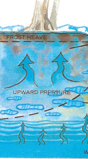
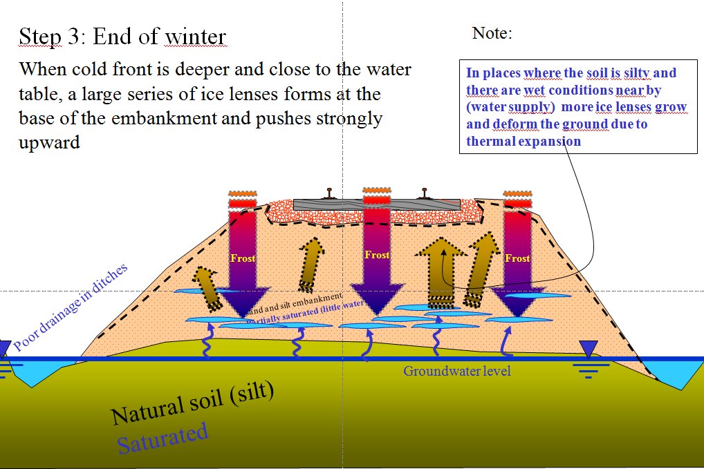
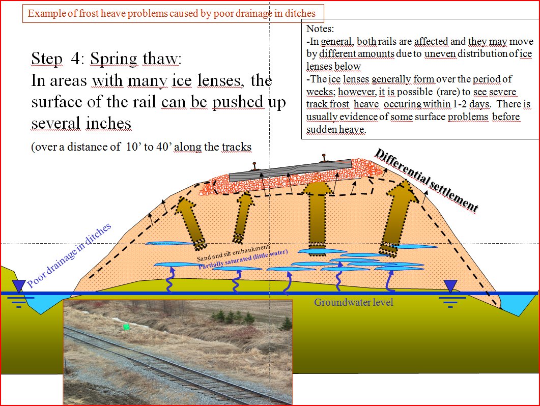
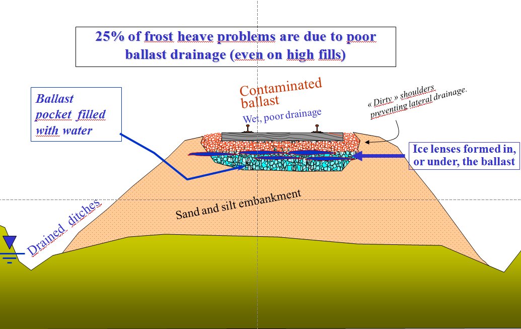
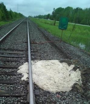
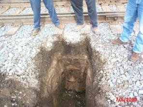
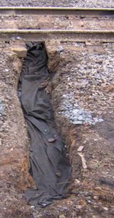
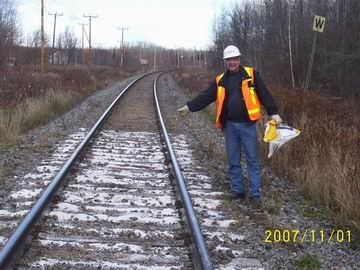
After Geotechnology for Railroaders Program, Module 6.6; §02–05. Full reference under Supplemental Sources.
If the subgrade is not stable, the track will not hold alignment, surface or cross level, however much maintenance is spent on it. Settle the subgrade before the track section. Investigate the alignment (Chapter 5). Design cuts, fills and subgrade preparation to AREMA Chapter 1, Part 2. Confirm soil suitability against the AREMA table of soil types and their suitability as railroad subgrade.
For cohesive subgrades, UFC 4-860-01FA sets the design bearing capacity of the track structure from the unconfined compressive strength, qu, measured at natural water content:
| Annual traffic | Design bearing capacity | Approximate equivalent |
|---|---|---|
| Less than 5 MGT | qu | 2 su |
| 5 MGT or more | 0.8 qu | 1.6 su |
Use as a screening check only. The UFC rule was written for low-tonnage installation track. The progressive-shear check in §2.5.1 (FS ≥ 3 on (π + 2) su) allows a stress of about 1.7 su divided by the dynamic load factor, so the UFC rule is less conservative. Use it to screen industry, yard and light-density branch-line track. For mainline and heavy-haul track, design to §2.5.1 and the granular layer methods in §2.4.
Chemical stabilization in frost areas. Use lime or cement stabilized subgrade under track with caution in seasonal-frost areas, and only after laboratory testing that includes frost susceptibility and freeze–thaw durability (Chapter 17, §17.7).
After UFC 4-860-01FA (2004), ch. 6, §8. Comparison with §2.5.1 added by the authors. Full reference under Supplemental Sources.
Track modulus (u) characterizes the stiffness of the combined track-subgrade system. It relates rail deflection to applied load:
u = P / (y × l_w) (lb/ft²)
In practice, track modulus is expressed as:
u = P_w / w_max (lb/ft of rail per in. of deflection)
where:
Typical track modulus values:
| Condition | u (lb/in./in.) | Equivalent (psi) |
|---|---|---|
| Soft subgrade, worn ballast | 1,000–2,000 | 7–14 |
| Average track, mixed subgrade | 2,000–4,000 | 14–28 |
| Good track, granular subgrade | 4,000–6,000 | 28–42 |
| High-quality concrete tie, stiff subgrade | 6,000–8,000 | 42–56 |
| Amtrak NEC high-speed standard | > 8,000 | > 56 |
Track modulus directly affects bending moment and deflection in the rail. The characteristic length:
l = (4EI / u)^(1/4) (in.)
where:
The maximum rail bending moment:
M_max = P_w × l / 4 (in.·lb)
Higher track modulus reduces deflection but increases dynamic impact forces. All Class I railroads target u ≥ 3,000 psi for 286K heavy-axle freight. Amtrak targets u ≥ 6,000 psi on the NEC.
McHenry and Rose (2012) reviewed the in-situ tests available for railroad subgrade. Beyond borings and CPT, the options most relevant to track modulus are:
Source: McHenry, M. and Rose, J. (2012). Railroad Subgrade Performance Indicators — A Review of Available Testing Methods. University of Kentucky
Profillidis expresses stiffness as a reaction coefficient ρ = load / settlement at the level considered (56 kip/in. per t/mm in the source). Typical component values are: rail 280,000–560,000 kip/in.; timber tie 50–80; concrete tie 1,200–1,500; ballast 10–30; rubber pad 560–1,120 kip/in.. The subgrade is the softest element in the chain:
| Subgrade | ρ (kip/in.) |
|---|---|
| Silty | 28–84 |
| Clay | 84–112 |
| Gravel or rock | 112–450 |
| Frozen | 450–560 |
Existing track with ballast only (no subballast): total ρ = 8.4–56 kip/in., average 17 kip/in.. Bridges: 560–840 kip/in..
| e (in.) | 0 | 6 | 8 | 12 | 16 | 20 |
|---|---|---|---|---|---|---|
| λ (subgrade stress ratio) | 1 | 0.70 | 0.50 | 0.35 | 0.25 | 0.20 |
| ρ / ρ0 | 1 | 1.40 | 2.00 | 2.85 | 4.00 | 5.00 |
Design should satisfy two principles: stresses reaching the subgrade must stay below failure values, and the track must remain flexible. A rock subgrade is more than three times as stiff as a clay subgrade, so even rock cuts need a full ballast and subballast section. In the finite-element breakdown (Figure 2-34), the subgrade supplies about 40–43% of total track elasticity, the track bed 20–22% and the rail pads 25–34%.
Figures · click to zoom
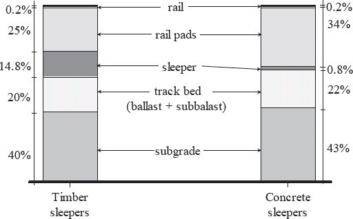
After Profillidis (2014), §8.2.2–8.2.3, §8.4.9, §8.8, Table 8.1, Figs. 8.12, 8.16. Full reference under Supplemental Sources.
Track modulus lumps the fastenings, ties, ballast, subballast and subgrade into one spring. It cannot be calculated from the components. It has to be measured. Selig and Waters describe three methods:
Remove slack. With all three methods, use the difference between a light seating load and a heavy load. This removes gaps and slack under the ties. Load–deflection curves are strongly nonlinear, and more so as track settles, so always report the load levels with the modulus.
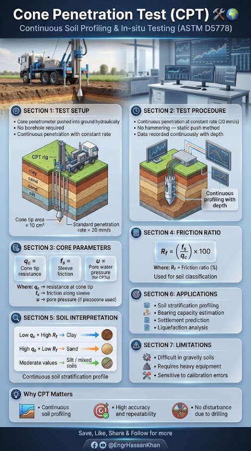
Field values and correlation. At eight U.S. sites, u ranged from 2,200 to 7,000 psi. CPT soundings to at least 16 ft below the tie, back-analyzed with a multilayer model, gave a subgrade resilient modulus of about Er ≈ 14 qc for all the data, or about 21 qc with outliers removed. This makes CPT a practical way to estimate track stiffness along a corridor.
Sensitivity. In the model, fastener stiffness had the largest effect on u, but it varies little in real track (about 10%). Ballast modulus, ballast depth, tie spacing and rail section each changed u by 10–20%. The subgrade remains the most influential variable in the field.
After Selig & Waters (1994), chs. 5 and 10. Full reference under Supplemental Sources.
Ballast fouling reduces drainage capacity and increases subgrade stress. The Fouling Index (FI) quantifies fouling:
FI = P₄ + P₂₀₀
where:
| FI Value | Fouling Condition | Recommended Action |
|---|---|---|
| < 1 | Clean | No action; monitor |
| 1–10 | Slightly fouled | Monitor; plan maintenance |
| 10–20 | Moderately fouled | Schedule ballast cleaning |
| 20–40 | Fouled | Immediate ballast cleaning |
| > 40 | Highly fouled | Ballast undercutting; possible subgrade work |
All Class I railroads track fouling condition through periodic ballast sampling programs. BNSF and UPRR Engineering Instructions require fouling index data to be included in geotechnical reports for mainline rehabilitation projects. GPR can estimate fouling condition non-destructively (Section 2.9).
Selig and Waters (1994) examined the source of fouling material at a large set of sites. Breakdown of the ballast itself was the major source at 76% of sites; upward migration from an underlying granular layer (usually old roadbed mixed in at the interface) was the major source at 13%. Contamination pumped up from the subgrade was rare. Li et al. point out that muddy ballast is often wrongly blamed on subgrade pumping when it is really ballast abraded under traffic in the presence of water — which changes the remedy from subgrade treatment to ballast renewal and drainage.
The Selig fouling index depends on the percent passing the No. 200 sieve, which is hard to measure reliably in the field. Canadian National uses the percent passing the ¾-in. sieve instead; Sussmann et al. (2012) matched the two scales:
Table 2-S4. Selig & Waters fouling index vs. CN ¾-in. sieve criterion
| Category | Fouling index (Selig & Waters) | % passing ¾ in. (CN) |
|---|---|---|
| Clean | < 1 | – |
| Moderately clean | 1 to < 10 | < 25 |
| Moderately fouled | 10 to < 20 | 25–40 |
| Fouled | 20 to < 40 | 40–50 |
| Highly fouled | > 40 | > 50 |
Table 2-S5. Ballast cleaning intervention limits used by different agencies
| Agency / source | Criterion | Limit | Basis |
|---|---|---|---|
| Selig & Waters | Fouling index | 40 / 30 | Highly fouled / drainage reduction |
| Spoornet | FISpoornet = 0.4P19 + 0.3P6.7 + 0.2P1.18 + 0.1P0.15 | 80 | Gradation change |
| Canadian National | % passing ¾ in. (¾ in.) | 40% | Highly fouled |
| UIC | % passing ½ in. (½ in.) | 30% | – |
| ERRI | % passing ⅞ in. (⅞ in.) | 30% | – |
For field sampling programs, the single-sieve CN criterion lets the crew classify a sample at the tie end without shipping it to the lab; reserve full gradations (and FI) for representative samples and design stations.
Source: Li, D., Hyslip, J., Sussmann, T. and Chrismer, S. (2016). Railway Geotechnics. CRC Press / Taylor & Francis
Figures · click to zoom
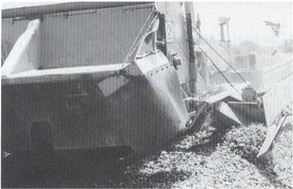
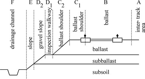
After Profillidis (2014), §12.7, §16.8–16.9, §16.12, §9.16, Figs. 9.21, 16.10. Full reference under Supplemental Sources.
Fouling comes mainly from particle breakdown under traffic, plus abraded tie material, spilled lading (coal, grain), wind-blown sand and silt, slurry pumped up from the subgrade, chemical weathering, and maintenance tools (tamping accelerates breakdown). Gradation testing shows a failure zone. Once material finer than ¾ in. passes about 25% (the ideal point to undercut) and heads toward 40% (action mandatory), degradation accelerates sharply, typically within 500 MGT. Ballast next to an active mud spot is usually near its own failure zone. Visual inspection is not enough; use sieve analysis or GPR.
| Method | Cost / duration | Result |
|---|---|---|
| Tamping | Low cost, very short term | Low efficiency: “tamping mud” |
| Skin lift | Low short-term cost | Out of the mud temporarily |
| Major lift | Medium | Longer term, but the problem may return |
| Shoulder cleaning | Medium | Better if ballast is not too fouled; can extend ballast life |
| Full-depth undercutting | High | Greatest gain in internal drainage and bearing; about 15 years at 50 MGT/year |
Undercut to about 12 in. below the ties, with the bar inclined to leave a 2% slope that drains to ditches or shoulders. Plan depths so every track drains on multiple-track territory, and place waste where it neither blocks drainage nor loads the shoulder. Undercutting without restoring lateral drainage gives minimal benefit. Watch for buried fiber. A documented move from reactive to planned ballast management cut ballast-related slow orders from over 600 to under 20 per year, ballast derailments from about 8 to about 0, and spending from over $250M to under $100M per year.
Figures · click to zoom
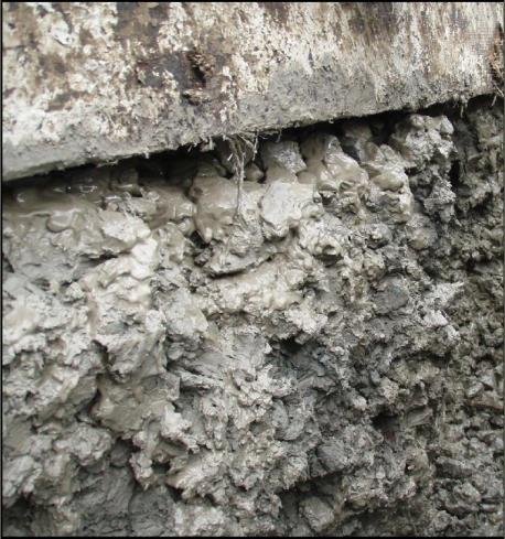
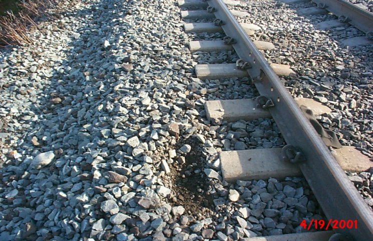
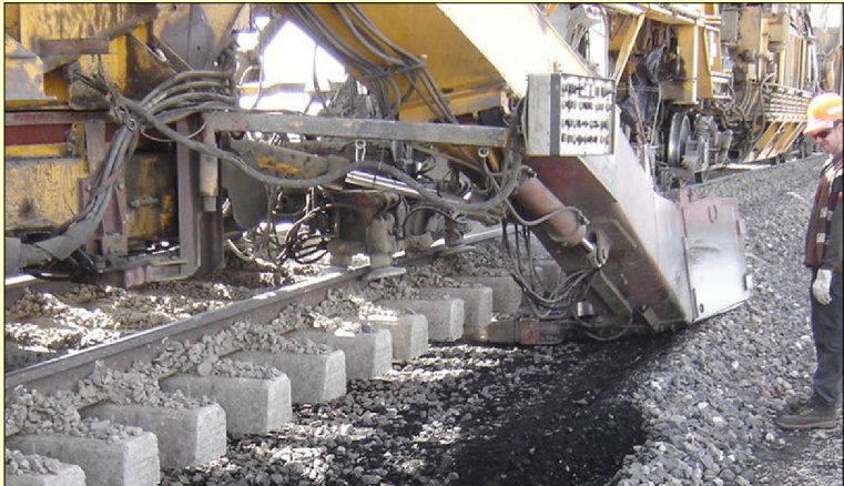

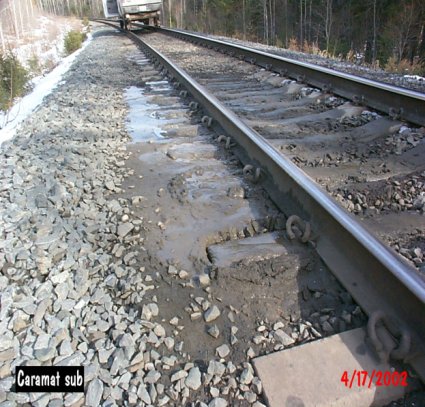
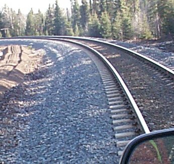
After Geotechnology for Railroaders Program, Module 3; §06–07, §13. Full reference under Supplemental Sources.
| Condition | Fouling index | kh, in./s | kh, mm/s |
|---|---|---|---|
| Clean | < 1 | 1–2 | 25–50 |
| Moderately clean | 1–9 | 0.1–1 | 2.5–25 |
| Moderately fouled | 10–19 | 0.06–0.1 | 1.5–2.5 |
| Fouled | 20–39 | 0.0002–0.06 | 0.005–1.5 |
| Highly fouled | ≥ 40 | < 0.0002 | < 0.005 |
Settlement. In box tests, settlement increased with fouling index. A small gap under the tie (0.039–0.16 in. of lift-off between loads) increased settlement by about an order of magnitude and accelerated both fouling and tie wear. Highly fouled ballast that settles quickly after tamping is a sign that it needs cleaning.
Sources vary by railway. British Rail attributed its fouling as follows:
North American sites were dominated by ballast breakdown (see above). Sample before assuming the source. In BR tests, 20 tamping insertions broke 15–45% of the 1½–2-in. particles, and each tamp produced 4–9 lb of material finer than ½ in.
Not all fines are equal. Sand and gravel fouling is tolerable. Silt forms an abrasive slurry. Clay fouling may require 100% ballast replacement.
Six ways to limit fouling:
Undercut or clean at a fouling index of about 40 if the ballast is cleanable. Plow or sled it out if it is fouled with wet, plastic fines.
After Selig & Waters (1994), chs. 8, 13 and 16. Full reference under Supplemental Sources.
Poor drainage is the single most common root cause of subgrade problems in North American railroad practice. The geotechnical consultant is responsible for assessing existing drainage adequacy and designing improvements.
Reference graphics · click to zoom
Required drainage capacity:
Q = C × i × A (ft³/s) [Rational Method]
where:
Subgrade drainage outlet spacing:
For a track grade of g (ft/ft) and allowable ponding width w (ft):
L_outlet = (w × k_subballast) / (i_net) (ft)
where k_subballast = lateral permeability (ft/day); i_net = net lateral hydraulic gradient.
In practice, AREMA Chapter 1 recommends longitudinal drainage outlets every 300–500 ft for typical mainline conditions; 150–200 ft for sag vertical curves.
Perforated pipe edge drains at the base of the subballast layer are required for all new mainline construction by CSXT, NSR, UPRR, BNSF, and CN engineering standards. Design:
Pipe diameter: 4 in. minimum perforated HDPE; 6 in. for grades < 0.5%
Filter requirements: Geotextile wrapping per AREMA Chapter 1 AOS requirements:
AOS ≤ D₈₅(subballast) (no piping)
k_geotextile ≥ 10 × k_subballast (adequate flow)
Reference graphics
UIC guidance is that the groundwater level should be at least 2.6 ft below the top of subgrade. Where it is not, it must be lowered with ditches or deep drains. Individual railways set their own minimum depths below rail or formation (Figure 2-37). Even where groundwater is deep enough, hydrogeological conditions are not rated “good” unless drainage devices are provided and the top of subgrade has a 3–5% crossfall. Sites with large seasonal groundwater fluctuation need a separate study, where a sand filter or geotextile may be warranted.
Geotextiles (polypropylene or polyester, 0.016–0.12 in. thick, woven or non-woven) separate, reinforce, filter and drain. They go under the subballast, never directly under the ballast. They do not replace ballast or subballast for load spreading: railways that laid a geotextile and also cut ballast thickness or omitted subballast saw the ballast puncture the fabric and lost the crossfall. A finite-element study found about a 10% reduction in stress at the top of subgrade from the geotextile. Filter permeability criteria quoted by the book:
where kg = geotextile permeability (ft/day), tg = geotextile thickness (in.), ks = soil permeability (ft/day) and d50 = soil 50% passing size (in.).
Figures · click to zoom
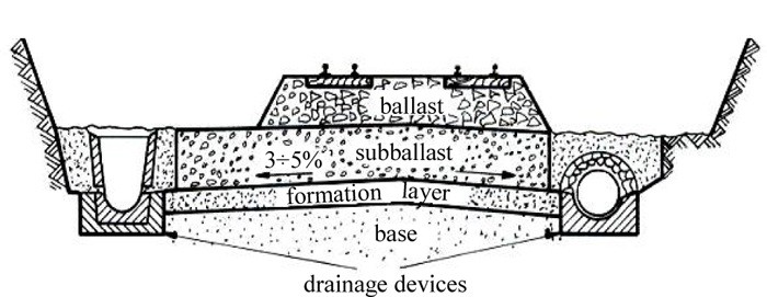
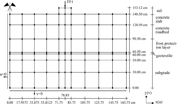
After Profillidis (2014), §9.4, §9.14.1, §9.15, Eqs. 9.13–9.14, Figs. 9.3, 9.4, 9.20. Full reference under Supplemental Sources.
On double track, each track drains laterally away from the centerline. On three or more tracks, the outside tracks drain outward and the inner tracks drain into longitudinal trench drains, with the subgrade and sub-ballast surfaces sloped to suit. Ballast-deck bridges need their own designed drainage. Lateral drainage blocks when there is no cross-slope, when ballast pockets have formed, or when material and vegetation build up between the ballast toe and the ditch. Water trapped in the ballast is the leading cause of mud-fouled ballast. Groundwater seepage, where the subgrade sits at or below a fluctuating water table, is the second.
Figures · click to zoom


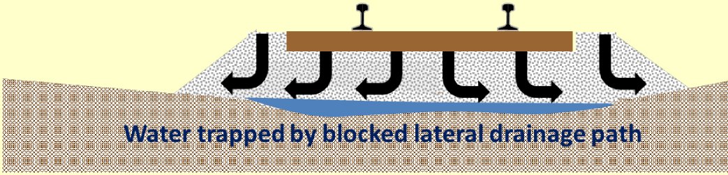

After Geotechnology for Railroaders Program, Module 4; §03, §05–06. Full reference under Supplemental Sources.
Three requirements. Track drainage works only if all three are met:
Size the system for the highest inflow expected over its design life, not the average.
The center of the track ponds first. On a low-permeability subgrade, water flows mostly sideways. About two-thirds of it leaves through the shoulders. The zone within about 12 in. of the track centerline has the longest flow path and saturates first, so it sets the critical rainfall rate.
Table 2-SW5 gives the critical rainfall rate for several ballast conditions. The cases assume 12 in. of ballast below the tie and 6 in. of silty-sand subballast on an impermeable subgrade.
| Ballast condition | Critical rate, in./hr |
|---|---|
| Clean | 5.9 |
| Clean shoulders; fouled (FI 30) below | 1.4 |
| Undercut, over FI 30 ballast | 0.33 |
| Undercut, over FI 40 ballast | 0.31 |
| Fouled throughout (FI 30) | 0.06 |
| Clean shoulders; highly fouled (FI 40) below | 0.02 |
| Highly fouled throughout (FI 40) | 0.001 |
Double track that drains to one side only has about half these critical rates.
How to use it.
After Selig & Waters (1994), ch. 13. Full reference under Supplemental Sources.
Case study: 2.18.2 Rail formation on broken hard rock: ruts after a week, tests all passed (Look 2023), in §2.18 Case Studies.
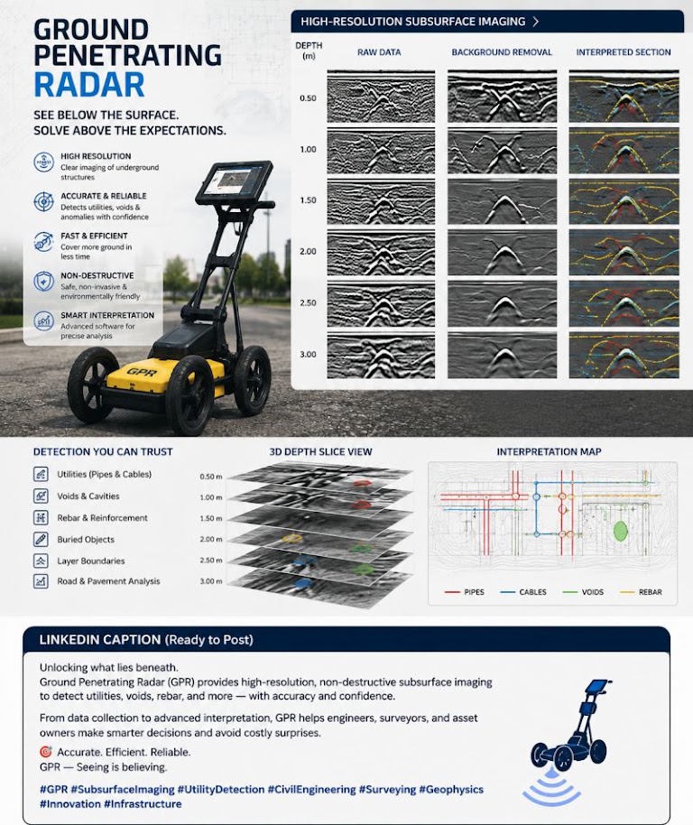
GPR is an efficient, non-destructive tool for mapping ballast fouling, subballast thickness, and subgrade moisture conditions along track. It is standard practice for mainline rehabilitation investigations at CSXT, NSR, UPRR, BNSF, and CN.
GPR uses an antenna (typically 400 MHz or 1 GHz) mounted on a hi-rail vehicle to transmit and receive electromagnetic pulses through the track structure. Reflections at material boundaries provide:
Reference graphics
The depth to a reflector:
d_GPR = (v × t_twtt) / 2 (ft)
where:
| Material | ε_r | Wave Velocity (ft/ns) |
|---|---|---|
| Clean granite ballast | 5–6 | 0.402–0.440 |
| Moderately fouled ballast | 8–12 | 0.284–0.348 |
| Highly fouled/saturated | 15–30 | 0.180–0.254 |
| Subballast (granular, dry) | 6–9 | 0.328–0.402 |
| Clay subgrade (moist) | 20–40 | 0.156–0.220 |
| Ballast voids/air | 1 | 0.984 |
Standard GPR deliverables for railroad geotechnical investigations:
CSXT Engineering Standards Section 6 and BNSF Engineering Instructions both require GPR survey results to be correlated with at least 10% field-verified boring data before design recommendations are finalized.
Leng and Al-Qadi measured the dielectric constant of granite and limestone ballast in a 36-in.-deep test box using 2-GHz air-coupled antennas (the same setup used on the BNSF Orin Subdivision validation data). Key findings useful when reviewing a GPR vendor’s interpretation:
Source: Leng, Z. and Al-Qadi, I. L. “Railroad Ballast Evaluation Using Ground-Penetrating Radar: Laboratory Investigation and Field Validation.” Transportation Research Record
| Railroad | Min. Ballast Depth (in.) | Min. Subballast (in.) | Blanket Layer | GPR Required? | FI Threshold | Governing Std. |
|---|---|---|---|---|---|---|
| CSXT | 12 (tie bottom) | 6 | Yes if CBR < 5 | Mainline rehab | FI > 20 | CSXT Eng. Std. Sec. 6 |
| NSR | 12 | 6 | Yes if CBR < 5 | Mainline rehab | FI > 20 | NSR Eng. Std. Sec. 6 |
| G&W | 10 | 6 | Case-by-case | Not required | FI > 25 | G&W Eng. Bulletin |
| UPRR | 12 | 8 | Yes if CBR < 4 | Mainline rehab | FI > 20 | UPRR Eng. Instr. Manual |
| BNSF | 12 | 8 | Yes if CBR < 4 | Mainline rehab | FI > 20 | BNSF Eng. Instructions |
| CPKC | 12 | 8 | Yes (frost design) | Mainline rehab | FI > 20 | CPKC Track Standards |
| Amtrak | 14 | 10 | Yes if CBR < 6 | All projects | FI > 15 | Amtrak Eng. Std. |
| CN | 12 | 8 | Yes (frost design) | Mainline rehab | FI > 20 | CN Eng. Standards |
| AREMA Min. | 10 | 6 | Per design | Case-by-case | FI > 20 | AREMA MRE Ch. 1 |
Project context: BNSF Powder River Basin mainline rehabilitation. Track carries unit coal trains at 286K GRL. Existing ballast depth averages 18 in.; subballast is 6 in. Client requests evaluation of subgrade adequacy.
Given:
Step 1: Dynamic wheel load
P_d = P_w × DLF = 40,000 × 1.4 = 56,000 lb
Step 2: Effective area at top of subgrade
A_eff = (0.917 + 2 × 2.0 × 0.700) × (8.5 + 2 × 2.0 × 0.700)
= (0.917 + 2.800) × (8.5 + 2.800)
= 3.717 × 11.300 = 42.0 ft²
Step 3: Vertical stress at top of subgrade
σ_s = P_d / A_eff = 56,000 / 42.0 = 1,333 psf = 0.67 tsf
Step 4: Check against subgrade capacity
Field vane shear tests on subgrade soil: s_u = 350 psf (average of 5 VST readings)
σ_allow = (π + 2) × s_u / 3.0 = 5.14 × 350 / 3.0 = 599 psf
FS = σ_allow / σ_s(static) = 599 / (40,000/42.0) = 599 / 952 = 0.63 < 1.0
The subgrade is critically overstressed even without dynamic amplification. Conclusion: Subgrade improvement is required. Minimum required total thickness to reduce σ_s(static) ≤ 599 psf: from Table 2-1, d ≥ 30 in. of ballast + subballast. BNSF standard is 12 in. ballast + 8 in. subballast = 20 in. total, which is insufficient. Recommend 24 in. ballast + 12 in. granular blanket (= 36 in. total), providing σ_s(static) = 400 psf < 599 psf ✓, or evaluate PVD + preloading per Chapter 17.
Project context: CSXT Georgia Division mainline at MP 42.3, reported for track geometry deviation. Ballast samples collected at 500-ft intervals over a 2-mile segment.
Given (representative sample at MP 42.3):
Step 1: Fouling Index
FI = P₄ + P₂₀₀ = 14.2 + 3.8 = 18.0
Per Table 2-5: FI = 18.0 → Moderately Fouled. CSXT threshold is FI > 20 for immediate action; this sample is approaching threshold.
Step 2: Assess along-alignment pattern
| MP | P₄ (%) | P₂₀₀ (%) | FI | Condition |
|---|---|---|---|---|
| 42.0 | 8.5 | 1.2 | 9.7 | Slightly fouled |
| 42.3 | 14.2 | 3.8 | 18.0 | Moderately fouled |
| 42.6 | 22.1 | 5.7 | 27.8 | Fouled |
| 42.9 | 31.4 | 9.2 | 40.6 | Highly fouled |
| 43.2 | 18.7 | 4.3 | 23.0 | Fouled |
| 43.5 | 11.1 | 2.6 | 13.7 | Moderately fouled |
Conclusion: The segment from MP 42.6 to MP 43.2 (0.6 miles) requires immediate ballast cleaning or undercutting. MP 42.9 (FI = 40.6) is at the threshold for undercutting with subgrade investigation. Recommend advancing 3 borings at MP 42.9 to assess whether ballast pockets have developed.
Step 3: Track modulus check at MP 42.9
At highly fouled locations, track modulus typically drops to < 2,000 psi. CSXT Engineering Standards require minimum u = 3,000 psi for Class 4 mainline. Confirm with deflection measurement (Hy-Rail mounted optical or accelerometer system).
Project context: CN Prairie North Line through Manitoba clay (Lac du Bonnet till, FS-3 subgrade). Track geometry defects occur each spring. Evaluate adequacy of existing 12-in. ballast + 6-in. subballast and design required blanket layer.
Given:
Step 1: Frost penetration in current section (Modified Berggren)
For granular fill above subgrade:
X = λ × √(FI_surface)
Using CN parameters: λ = 1.50 ft/°F·days^0.5 (average for granular fill, from Chapter 18 climate table)
X = 1.50 × √2,800 = 1.50 × 52.9 = 79.4 in. = 6.6 ft
The 32°F isotherm penetrates 6.6 ft below top of ballast. Current non-frost-susceptible layer is only 1.5 ft. The isotherm enters native till at 1.5 ft depth.
Step 2: Required blanket thickness
Required non-frost-susceptible fill to intercept freezing front:
d_blanket ≥ 6.6 ft − 1.5 ft (existing) = 5.1 ft additional blanket layer
This is impractical as a strictly thermal solution. CN Engineering Standards permit use of XPS insulation board (R-10 per inch, min. 2 in. thick) to reduce required fill thickness.
With 2 in. XPS insulation (thermal equivalent to 2.5 ft granular fill):
d_blanket = 6.6 ft − 1.5 ft − 2.5 ft (insulation equivalent) = 2.6 ft granular blanket (31 in.)
Conclusion: Provide 31 in. of FS-0/FS-1 granular blanket + 2 in. XPS insulation board below existing subballast. Verify that final σ_s at top of subgrade (including blanket) satisfies bearing capacity. CN Engineering Standards require frost blanket designs to be submitted with PE seal.
| Station | Client | Subgrade USCS | s_u (psf) | CBR | FI | d_total (in.) | σ_s (psf) | FS_shear | GPR Anomaly |
|---|---|---|---|---|---|---|---|---|---|
| A+00 | BNSF | CH | 350 | 1.8 | N/A | 20 | 1,333 | 0.63 | Mud pocket |
| B+50 | CSXT | SC | 620 | 4.2 | 18.0 | 24 | 900 | 2.09 | Moderately fouled |
| C+00 | NSR | ML | 480 | 3.1 | 27.8 | 24 | 900 | 1.62 | Fouled zone |
| D+25 | CN | CL | 290 | 1.5 | N/A | 18 | 2,190 | 0.40 | Wet subgrade |
| E+75 | Amtrak | SP | 750 | 8.5 | 9.7 | 30 | 660 | 3.45 | Clean |
| F+00 | G&W | SM | 900 | 6.8 | 13.7 | 24 | 900 | 3.03 | Slightly fouled |
| G+50 | CPKC | ML | 420 | 2.8 | N/A | 18 | 2,190 | 0.58 | Frost lens |
| Material | E (psi) | Poisson’s ν | c (psi) | φ (°) |
|---|---|---|---|---|
| Poor subgrade (S1) | 1,780 | 0.4 | 2.1 | 10 |
| Medium subgrade (S2) | 3,560 | 0.3 | 1.4 | 20 |
| Good subgrade (S3) | 11,400 | 0.3 | 0 | 35 |
| Rock subgrade (R) | 427,000 | 0.2 | 210 | 20 |
| Ballast | 18,500 | 0.2 | 0 | 45 |
| Gravel subballast | 28,400 | 0.3 | 0 | 35 |
| Sand | 14,200 | 0.3 | 0 | 30 |
Values converted from kp/cm² by the authors (1 kp/cm² = 14.22 psi). These are model inputs from UIC test programs, not design values for a specific site.
The cross-sections below show the European layering in practice: 3–5% crossfall on the subballast and subgrade, 2:3 ballast and fill side slopes, and 12 ft track centers to the edge of the formation on a double track with drains and signal/electrification foundations at the shoulder.
Figures · click to zoom
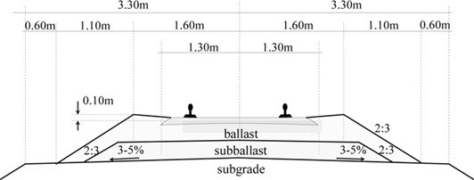
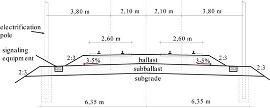
After Profillidis (2014), §8.4.6, Table 8.2, §12.6, Figs. 12.7, 12.9. Full reference under Supplemental Sources.
Reference graphics
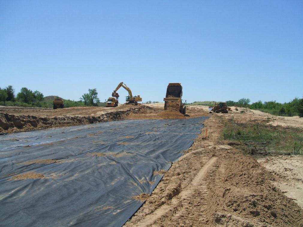
Source: Herbert, D. and Gee, B. (2021). “Durability and Performance of Geogrid-Stabilized Ballast and Sub-ballast Track Section in Mobile, Alabama.” AREMA 2021 Annual Conference · Coleman, D. M. (1990). Use of Geogrids in Railroad Track: A Literature Review and Synopsis. U.S. Army Engineer Waterways Experiment Station, Misc. Paper GL-90 · Getzner Werkstoffe. Sub-Ballast Mats (product technical brochure)
ASCE (2012) describes the owner’s resident project representative (RPR) as the person or firm that administers the construction contract on the owner’s behalf. RPR duties may include performing or directing QA, monitoring expenditures and progress payments, pushing timely review of submittals by the designer, evaluating and deciding on unforeseen conditions, coordinating owner site activities such as safety monitoring and testing, building the project record, and negotiating change orders.
The Manual divides materials into two classes. In situ materials are the native soil and rock; their suitability is established by laboratory testing and engineering evaluation, and the results and any retesting go into the project file. Procured materials include natural products such as earth fill and aggregates as well as manufactured items. For each procured material the file should record the qualification procedure and acceptance criteria, test type and date, the signature of the person testing, results, any nonconformance reports and, where specified, where in the structure the tested material was placed. Where workmanship is critical, the contractor may build a mock-up that, once accepted, becomes the standard for the remaining work. Substitutions are accepted only after the designer confirms they meet project objectives, and are then formalized by change order.
On unit-price contracts, common where quantities cannot be known precisely, the RPR and contractor jointly measure completed quantities. The Manual acknowledges that unknown soil conditions can change quantities enough that a unit price must be renegotiated, sometimes with a change in contract time. On lump-sum work the RPR checks that the schedule of values is not unbalanced.
For railroad work: Ballast, subballast, geosynthetics and select fill are procured materials and should be accepted against the railroad’s specification with traceable test records tied to stockpile, delivery ticket and placement station. Native subgrade exposed by undercutting is an in situ material whose acceptance (or further undercut) depends on the engineer’s evaluation at the time, which is a natural role for the RPR. A short test section at the start of a subgrade rehabilitation, accepted on proof rolling and density, can serve as the mock-up that sets the standard for the rest of the work.
Source: American Society of Civil Engineers (2012). Quality in the Constructed Project: A Guide for Owners, Designers, and Constructors, 3rd ed. ASCE Manuals and Reports on Engineering Practice No. 73. Reston, VA: ASCE, pp. 169–175. Summarized and paraphrased. Full reference under Supplemental Sources.
Function analysis is the core of value management. It describes what a project or element must do, as two-word verb–noun pairs, before anyone discusses what it should be. Kelly, Male and Graham have a team brainstorm functions, sort them from high-order needs down to low-order wants, and arrange them in a FAST (Function Analysis System Technique) diagram. Read left to right, the diagram answers “how?”; read right to left, it answers “why?”. A scope line separates the project’s mission from the functions open to brainstorming. In their technical FAST for a river crossing in a park, the mission “facilitate passage across river” leads to the primary function “support people,” with the parallel function “span river” and secondary functions such as “protect people” and “control people.” Design objectives such as “non-slip surface” and “reduce downtime due to flooding” sit above the diagram. Because the team works from functions, the solutions it considers range beyond bridge types: the authors note the answer might be a cable ferry rather than a bridge. For elements, element function analysis has five stages: pick the cost-dominant elements; list every function the element can perform; delete the functions not needed in this context; brainstorm against the functions that remain; and evaluate.
For railroad work: Apply element function analysis to the track substructure before choosing a remedy for a chronic soft spot. The candidate functions of ballast, subballast and subgrade include “distribute load,” “resist shear,” “drain water,” “separate layers,” “restrain track,” “limit frost penetration” and “provide resilience.” Keep only those the investigation shows are failing. If the evidence points to failed “drain water” and “separate layers,” that is, mud-pumping fines with a sound deeper subgrade, the brainstorm should center on drainage and filter or separation solutions, not a deep undercut. If “resist shear” is failing in the subgrade itself, the option set changes. Stating the needed functions explicitly ties the recommendation to the diagnosis and gives reviewers a clear reason why other remedies were set aside.
Source: Kelly, J., Male, S. and Graham, D. (2004). Value Management of Construction Projects. Oxford: Blackwell Science, pp. 62–69, 75–77. Summarized and paraphrased; figures reproduced for internal reference. Full reference under Supplemental Sources.
Passeck’s chapter in Jacob and Müller builds earthwork unit prices from the bottom up. The direct cost of each bid item is split into five parts: labor, equipment (including fuel and lubricants), materials, third-party services and transport, and site facilities. Percentage surcharges are then added. The example uses 8% general overhead, 6% site overhead, 3% risk and 3% profit, a total of 20%.
The cost components are built up as follows:
Worked haul example (book values converted to US units):
The excavate-haul-place-compact item then added loading (14%), haul (57%), spreading and compaction with one dozer and two rollers (25%), and fine grading (4%). Haul dominated the cost.
The authors stress pricing all earthwork items together, using a mass haul diagram to minimize haul distance and stockpiling, and adjusting manufacturer production figures for soil class, swell and site constraints.
For railroad work: Undercutting and subgrade rehabilitation estimates should be built the same way. The cycle is constrained by track-window length, the number of access points, and on-track or hi-rail haul instead of open haul roads. Haul units cannot cross or foul the live track without protection. Use productivity per effective window hour after setup, flagging and clearing time, not per shift hour. Show spoil disposal (especially fouled ballast) and imported subballast as separate cost lines.
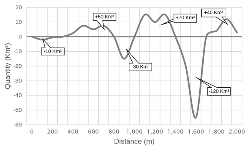
Source: Jacob, D. and Müller, C. (Eds.) (2017). Estimating in Heavy Construction: Roads, Bridges, Tunnels, Foundations. Berlin: Ernst & Sohn, pp. 36–50. Summarized and paraphrased; figures reproduced for internal reference. Full reference under Supplemental Sources.
Pratt prices excavation from productivity and crew cost, and keeps the two separate. Unit cost equals crew-hours per unit times cost per crew-hour. That way a change in wage rates and a change in productivity can each be applied on its own. Applied separately, an 8% wage increase and a 10% productivity loss raise the unit price by 18.8%, not the 18% you get by adding them.
Fixed costs depend heavily on job size. A backhoe that digs 60 CY/h, with $4,000 for transport and set-up, comes to $2.73/CY for equipment on a 3,000-CY job but $14.73/CY on a 300-CY job.
For hauling, Pratt sizes the truck fleet so that the excavator or loader never waits:
Number of trucks = (round-trip travel time + unloading time) / loading time + 1, always rounded up
Loading time is the truck’s bank-measure capacity divided by the loader output. Bank capacity is the loose capacity divided by (1 + swell). In his gravel example, the pit is 16 miles away, trucks average 20 mph and take 5 minutes to unload, so the cycle away from the loader is 101 minutes. A 12-CY truck with 12% swell carries 10.71 bank CY. At 50 BCY/h the loader fills it in 12.85 minutes, so the fleet is 101/12.85 + 1 = 8.86, rounded up to 9 trucks. With a $2.50/CY pit royalty, the delivered gravel costs $16.34 per bank CY. A price quoted per ton is converted using the weight of a compacted cubic yard: $/CY = $/ton × (lb/CY) / 2,000.
Table 2-PM2. Table: Loose and bank weights and compaction factors (after Pratt 2011, Figure 10.2)
| Material | Loose (lb/CY) | Bank (lb/CY) | Compaction factor |
|---|---|---|---|
| Clay, dry | 2,500 | 3,100 | 24.0% |
| Gravel, pit-run, dry | 2,550 | 2,850 | 11.8% |
| Sand, dry | 2,400 | 2,700 | 12.5% |
| Sand and gravel, dry | 2,900 | 3,250 | 12.1% |
For railroad work: on undercutting and subgrade rehabilitation, the track window usually sets the production rate, not the excavator. Estimate the cubic yards that can be removed and replaced per window. Then size the spoil trucks, side-dump cars or ballast cars with Pratt’s formula, so the machine never waits during a window that has already been paid for. On short jobs, fixed costs (mobilization, work-train set-up, flagging) are spread over a small quantity and dominate the unit price, as Pratt’s 300-CY case shows. Price imported subballast in bank measure, with explicit compaction and waste allowances.
Source: Pratt, D. J. (2011). Fundamentals of Construction Estimating, 3rd ed. Clifton Park, NY: Delmar Cengage Learning, pp. 224–235. Summarized and paraphrased. Full reference under Supplemental Sources.
Checklist · Part III · Track Substructure
Investigation Phase
Analysis and Design Phase
Deliverable Phase
| Topic | See Also |
|---|---|
| CBR and subgrade M_r testing | Chapter 18 |
| Frost blanket design (Modified Berggren) | Chapter 18, Section 18.6 |
| Ground improvement for soft subgrade | Chapter 17 |
| Undrained shear strength from VST/CPT | Chapter 7 |
| Consolidation settlement of subgrade | Chapter 12 |
| Bearing capacity of subgrade layer | Chapter 11 |
| Geotechnical Special Provisions (subgrade) | Appendix C |
| Lab testing for subgrade soils | Chapter 10 |
Q1. A concrete tie track carries Cooper E-80 loading with DLF = 1.3. Ballast depth is 14 in. (1.167 ft) and subballast is 8 in. (0.667 ft), giving d = 1.833 ft. Tie width B_t = 11 in. (0.917 ft), L_t = 8.5 ft. Calculate: (a) dynamic wheel load P_d, (b) effective area A_eff at top of subgrade (θ = 35°), and (c) vertical stress σ_s.
Answer:
Q2. A subgrade soil has s_u = 500 psf (from VST). The static wheel load is 40,000 lb and A_eff = 42.0 ft². (a) Calculate σ_s(static). (b) Calculate allowable stress for cyclic loading (FS = 3.0). (c) Is the subgrade adequate? (d) What total layer thickness d would reduce σ_s(static) to σ_allow?
Answer:
Q3. A ballast sample has 17.5% passing No. 4 sieve and 4.2% passing No. 200 sieve. (a) Calculate Fouling Index. (b) What is the fouling classification? (c) What action is recommended by BNSF Engineering Instructions?
Answer:
Q4. A rail section uses 136 RE rail (I = 95.0 in.⁴, E = 30 × 10⁶ psi) and has a track modulus u = 2,500 psi. (a) Calculate the characteristic length l. (b) Calculate the maximum rail bending moment under P_w = 40,000 lb.
Answer:
Q5. A GPR survey identifies a reflector at t_twtt = 8.5 ns in ballast with estimated ε_r = 6.5. (a) Calculate the wave velocity in this ballast. (b) Calculate the depth to the reflector. (c) If the expected ballast/subballast interface is at 24 in. (2.0 ft), is the measured depth consistent with a clean or fouled ballast layer?
Answer:
Field case studies by Burt G. Look, from Earthworks: Theory to Practice – Design and Construction (CRC Press/Balkema, 2023), chosen for this chapter’s topics. Each is summarized from the book with its key figures and a closing note on railroad application added by the authors of this manual. Credit for the case material belongs to Look; see item S13 under Supplemental Sources.
Related section: 2.4 Subballast Requirements and Blanket Layer Design
In a 2008 rail project, residual soils in Cut No. 5 (about 40,500 yd³) had their highest CBR in the middle of the cutting, not at depth. Strength does not necessarily increase with depth. Using the CBR 10 material at subgrade level would have reduced layer thickness and the imported capping layer, here the subballast, so it was stockpiled for reuse.
Checks on the stockpile found inconsistent CBR, and inspection showed it had been mixed with poorer material, visible as a change in colour. Look’s shorthand for the result: CBR 10 + CBR ≤ 5 ≠ CBR 7; the mix behaves more like CBR 5.
For railroad work: selective excavation and zoning can cut subballast quantities, but only with stockpile control: separate, marked piles, a haul plan, and verification testing of the stockpile before it is placed. Without that, design the subballast for the poorer material.
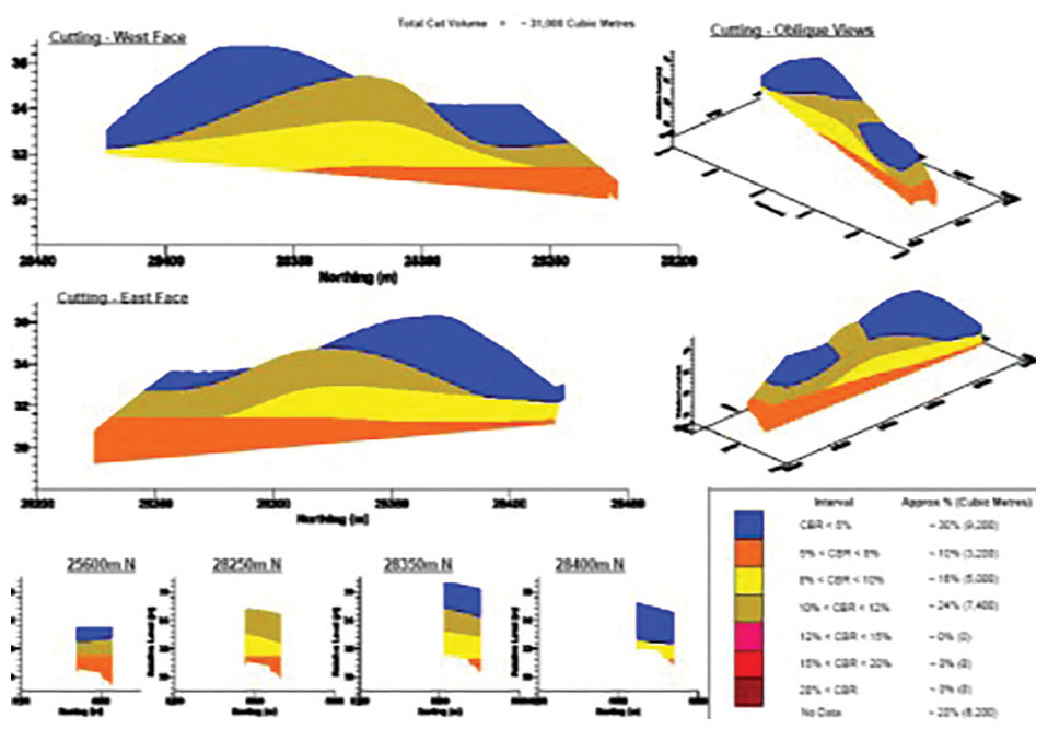
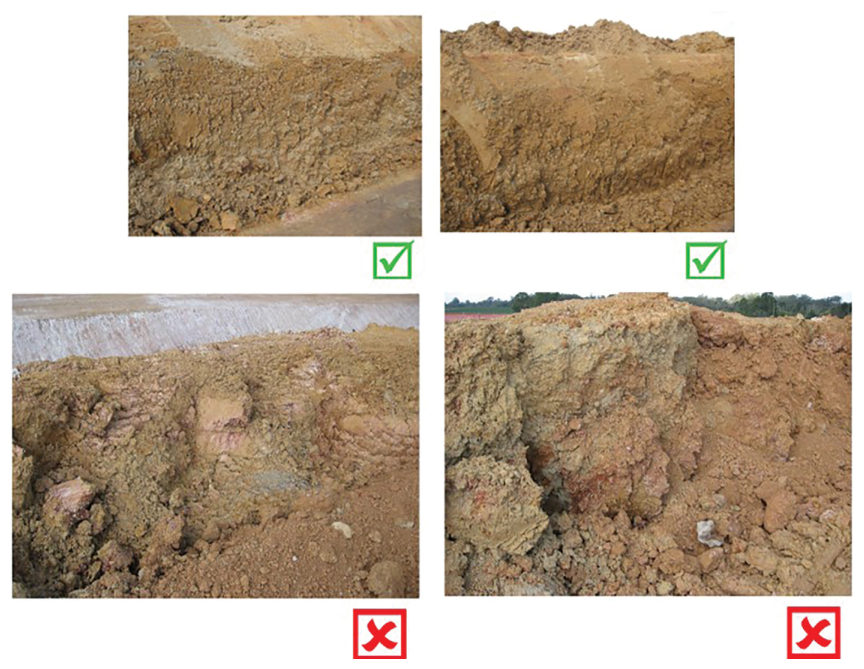
Source: Look, B. G. (2023). Earthworks: Theory to Practice – Design and Construction. CRC Press/Balkema. Case study §14.15, pp. 552–554. Summarized and paraphrased; figures reproduced for internal reference. Full reference under Supplemental Sources.
Related section: 2.8 Subgrade Drainage Design
On a 3.7 mi rail alignment around 2008, a short cutting (under 490 ft) hit very high-strength volcanic rock near the surface. With small volumes and no other large cuts, the contractor used a rock breaker, and the work took more than six months. The broken rock surface was uneven and out of tolerance for the required vertical grade. High-quality fill was compacted into the voids to even it out before the capping layer was placed.
Rain followed soon after. No ponding showed at the surface, but water collected in the hollows of the impermeable rock below and could not drain. About a week after completion, construction traffic rutted the formation, although the density and plate load tests had passed. With water trapped in these “bowls”, Skempton’s B is about 1, so each truck pass generated high excess pore pressure. Look’s lessons:
For railroad work: the same trapped-water mechanism produces mud pumping and track geometry defects where subballast sits on an irregular rock or old hard-pan surface. Shape the rock formation to drain, or level it with lean concrete, before placing subballast.
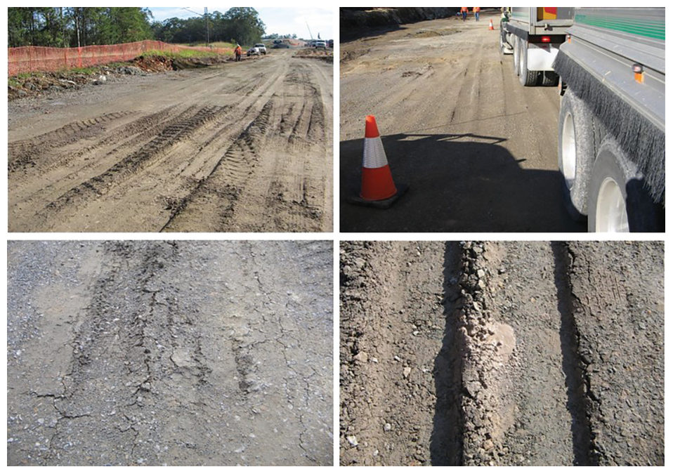
Source: Look, B. G. (2023). Earthworks: Theory to Practice – Design and Construction. CRC Press/Balkema. Case study §14.13, pp. 548–550. Summarized and paraphrased; figures reproduced for internal reference. Full reference under Supplemental Sources.
Authors: Daniel P. Colwell and Mario Ruel. This chapter was written and compiled by Daniel P. Colwell and Mario Ruel for Railway Ground Hazard Risk Management.
Technical content is drawn from the published sources below, and credit for that material belongs to their authors and publishers. Tables, equations and figures taken from a specific source are also cited where they appear.
File locations for these documents are listed under Supplemental Sources — LEVI Library.
Material in the green “Supplemental reference” boxes throughout this chapter was added from the following documents in the LEVI geotechnical library. Text is summarized or paraphrased; tables are reproduced with their original source noted; figures are reproduced from the cited document for internal reference use. Consult the original document before relying on a value for design. Blocks marked “After UFC 4-860-01FA (2004)” draw on item S11 and are rewritten for railroad clients. Blocks marked “After Selig & Waters (1994)” summarize item S12 for railroad clients; tables are condensed from the book and its figures are not reproduced. The Case Studies section summarizes case studies from item S13 by Burt G. Look; its figures are reproduced from the book for internal reference use, and the closing “For railroad work” note in each case study is added by the authors of this manual. Blocks tagged “Project management” summarize methods, examples and figures from the project-management, estimating and construction-management books listed here, applied to railroad work; the closing “For railroad work” note in each block is added by the authors of this manual.