
Geotechnical engineering libraryContact
Primary Reference: USACE EM 1110-1-1804, Geotechnical Investigations (January 2001); AASHTO Guide for Design of Pavement Structures (1993); AASHTO M 145-91; ASTM D1883 (CBR); ASTM D4318 (Atterberg Limits); ASTM D1621 (California Bearing Ratio); NCHRP Report 1-37A (M_r); AREMA MRE Chapter 1 (Track Structure); FRA Track Safety Standards 49 CFR Part 213.
Apps on dirtbert.com that support this chapter. Each one runs in a web browser on a desktop or a phone, with nothing to install. How to use the apps (I.3).
NANCY pages ask you to accept the Use and Disclaimers once in each browser.
Pavement subgrade evaluation for railroad facilities encompasses two distinct but related infrastructure domains: (1) paved surfaces within railroad right-of-way — intermodal container yards, locomotive servicing facilities, maintenance-of-way (MOW) vehicle access roads, classification yard roadways, and fueling pads; and (2) the granular track substructure system — ballast, subballast, and subgrade — which functions as an engineered pavement system for track loading. Both domains require rigorous characterization of subgrade support capacity, compressibility, moisture sensitivity, and frost behavior.
This chapter provides methods for characterizing subgrade strength (CBR, M_r, k modulus), designing flexible and rigid pavement structural numbers using AASHTO 1993 methodology, evaluating frost penetration and heave potential for CPKC and CN northern operations, and developing subgrade improvement recommendations for intermodal yard heavy container crane trackage. All equations are presented in English units. Railroad-client-specific pavement standards are integrated throughout.
Railroad pavement subgrade evaluation differs from highway pavement design in several important respects:
Loading regime: Intermodal yards subject paved areas to heavy rubber-tired container handlers (reach stackers up to 180,000 lb gross weight; loaded highway tractors at 80,000 lb GVW), overhead gantry crane rail loads (250–500 kip axle loads on crane rail foundations), and stacked container loads (4-high stacking of 45,000-lb gross containers = 180,000 lb per stack pad). These loads are far more severe than typical highway loadings and require higher subgrade strength criteria.
Crane rail foundations: Container cranes at intermodal yards ride on embedded crane rails set in reinforced concrete beams spanning pile caps. The geotechnical input — differential settlement between crane rail beams — governs structural crane serviceability more than pavement structural number alone.
Frost sensitivity: CPKC and CN operate intermodal terminals and MOW facilities in areas subject to frost depths of 4–8 ft (Prairie provinces, Manitoba, Ontario, Quebec, British Columbia interior). Subgrade frost heave of even 1–2 in. creates unacceptable differential movement in crane rails and reach stacker lanes.
Heavy industrial use: Unlike highway pavements rated by equivalent single axle loads (ESALs) over a 20-year design life, railroad intermodal pavement is often designed for 15-million-ESAL equivalents to reflect 24/7 terminal operations with heavy handling equipment.
Client-specific standards table:
| Railroad | Applicable Standard | Design Life (yr) | Target ESAL | CBR Minimum | M_r Minimum (psi) | Pavement Type Preferred | Notes |
|---|---|---|---|---|---|---|---|
| UPRR | UPRR EIM — Intermodal Facilities | 20 | 15M | 10 (improved) | 4,500 | JPCP rigid | Crane rail on pile caps; Omaha HQ review |
| BNSF | BNSF EI — Facility Engineering | 20 | 10M | 8 | 4,000 | HMA or JPCP | GIS facility asset management |
| CSXT | CSXT ES — Facility Pavement | 20 | 10M | 8 | 4,000 | HMA | Nashville/Jacksonville terminals |
| NSR | NSR ESM — Facility Design | 20 | 8M | 6 | 3,500 | HMA | Norfolk, Atlanta terminals |
| Amtrak | Amtrak ES — Station Facilities | 25 | 5M | 6 | 3,000 | JPCP or HMA | Passenger platform zones rigid |
| CPKC | CPKC TS — Intermodal Facilities | 25 | 10M | 10 (improved) | 4,500 | JPCP rigid | Frost depth design mandatory |
| CN | CN ES — Intermodal Standards | 25 | 12M | 10 (improved) | 4,500 | JPCP rigid | Prairie terminals; frost design required |
| G&W | AREMA + State DOT standards | 15 | 3M | 5 | 3,000 | HMA | Varies by short-line jurisdiction |
| AREMA | AREMA MRE Chapter 1 | 20 | Per design | 5 | 3,000 | Per owner preference | Minimum baseline |
JPCP = Jointed Plain Concrete Pavement; HMA = Hot-Mix Asphalt; ESAL = Equivalent Single Axle Load.
Reference graphics
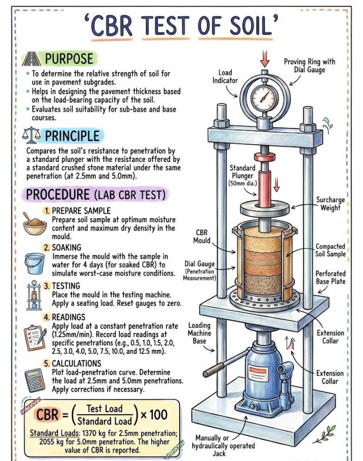
The CBR test (ASTM D1883 — laboratory; ASTM D4429 — field) measures resistance of a compacted soil to penetration by a standard cylindrical piston at a rate of 0.05 in./min. The CBR value is expressed as a percentage of the standard force required to penetrate a standard aggregate:
Where:
Soaked CBR (4-day immersion) is used for pavement design to simulate worst-case seasonal saturation. Unsoaked CBR may be used for check only.
| USCS Symbol | Soil Description | Typical CBR Range (%) | AASHTO Class | Suitability |
|---|---|---|---|---|
| GW, GP | Clean gravels | 40–80 | A-1-a | Excellent |
| GM, GC | Silty/clayey gravels | 20–60 | A-1-b | Good–Excellent |
| SW, SP | Clean sands | 10–40 | A-1-b, A-3 | Good |
| SM | Silty sands | 5–20 | A-2-4, A-2-6 | Fair–Good |
| SC | Clayey sands | 4–12 | A-2-6, A-2-7 | Fair |
| ML | Silt, sandy silt | 3–8 | A-4 | Poor–Fair |
| CL | Low-plasticity clay | 2–6 | A-6 | Poor |
| OL | Organic silt/clay | 1–4 | A-4, A-5 | Very Poor |
| MH | Elastic silt | 2–6 | A-5 | Poor |
| CH | High-plasticity clay | 1–4 | A-7-5, A-7-6 | Very Poor |
| OH, Pt | Organic clay/peat | < 2 | A-8 | Unsuitable |
Reference graphics
The resilient modulus is the fundamental subgrade input for AASHTO 1993 pavement design and NCHRP 1-37A (Mechanistic-Empirical Pavement Design):
Where:
ASTM T 307 laboratory testing applies a sequence of conditioning and test cycles at varying confining and deviator stresses. For preliminary design, M_r is estimated from CBR:
From Atterberg Limits (AASHTO T 274 regression for fine-grained subgrade):
Fine-grained resilient modulus depends on stress state, soil type and structure (compaction method), moisture and dry density. Selig and Waters give two relations for the modulus wet of optimum, with Δw = w − wopt in percentage points:
At 2 points wet of optimum these give about 0.54 and 0.63 (authors’ evaluation). That is roughly a 40–45% loss of stiffness. Use a wet-season moisture when selecting design Mr for track and yard subgrade.
After Selig & Waters (1994), ch. 10. Full reference under Supplemental Sources.
For rigid pavement (Portland cement concrete) design, the Westergaard modulus of subgrade reaction k (pci — lb/in.³) characterizes the support provided by the subgrade beneath the slab:
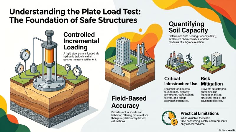
Plate load test (ASTM D1196): Apply load via 30-in. diameter bearing plate; record settlement at 0.05-in. increments:
Where p = applied pressure (psi) and δ = plate settlement (in.) at 0.1-in. target penetration.
Correlation from CBR (Portland Cement Association):
Correlation from M_r:
| Soil Type | USCS | CBR (%) | k (pci) | M_r (psi) | Pavement Suitability |
|---|---|---|---|---|---|
| Gravel/gravel-sand | GW, GP | 40–80 | 535–1,070 | 15,000–30,000 | Excellent |
| Sandy gravel | GM, GC | 20–50 | 267–667 | 8,000–20,000 | Good |
| Sand, gravelly sand | SW, SP | 10–40 | 133–535 | 5,000–15,000 | Fair–Good |
| Silty sand | SM | 5–20 | 67–267 | 3,500–8,000 | Fair |
| Clayey sand | SC | 4–12 | 53–160 | 3,000–5,500 | Fair |
| Silt, sandy silt | ML | 3–8 | 40–107 | 2,500–4,500 | Poor–Fair |
| Low-plasticity clay | CL | 2–6 | 27–80 | 1,500–3,500 | Poor |
| High-plasticity clay | CH | 1–4 | 13–53 | 1,000–2,500 | Very Poor |
Reference graphics
The USACE PCASE desktop implements the Unified Facilities Criteria for pavements, including UFC 3-250-01 (roads, streets, walks and open storage areas) and UFC 3-250-09 (aggregate-surfaced roads). It is useful for container yards and laydown areas that fall outside AASHTO traffic assumptions. Its modules cover traffic (a vehicle database that can be edited for handlers and cranes), design by CBR or layered-elastic methods with seasonal sets and frost design, evaluation, FWD back-calculation, and a DCP module. The DCP module converts blows and penetration to CBR, k or modulus for a 17.6-lb or 10.1-lb hammer, with “all soils”, lean-clay or heavy-clay correlations. It breaks the profile into layers automatically, and the resulting layer structure can be imported directly into the evaluation module.
Source: U.S. Army Corps of Engineers (2010). PCASE 2.09 User Manual. Transportation Systems Center / ERDC
UIC links its subgrade quality classes (S0–S3) to ranges of modulus of elasticity and CBR (Figure 18-11). This lets CBR results from yard or access-road work be read against the track-subgrade classification in Chapter 2. Rock subgrades have moduli of the order of 430,000 psi. Profillidis defines CBR as the load producing 0.1 in. of penetration in the sample, divided by the load producing the same penetration in a standard reference material.
He adapts Dormon’s rule from highway engineering for the effect of traffic on subgrade stress: σ1/σ2 = (N2/N1)λ, with λ ≈ 0.2.
Figures · click to zoom
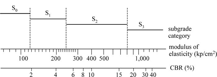
After Profillidis (2014), §9.6, §9.8, Fig. 9.5. Full reference under Supplemental Sources.
| Feel | Field indication | SPT (blows) | Shear strength (psf) | CBR |
|---|---|---|---|---|
| Very soft | Person standing sinks > 3 in. | < 2 | < 250 | < 0.4 |
| Soft | Person walking sinks 2–3 in. | 2–4 | 250–500 | 0.4–0.8 |
| Medium | Person walking sinks ~1 in. | 4–8 | 500–1,000 | 0.8–1.6 |
| Stiff | Pickup ruts 0.47–1 in. | 8–15 | 1,000–2,000 | 1.6–3.2 |
| Very stiff | Loaded dump truck ruts 1–3 in. | 15–30 | 2,000–4,000 | 3.2–6.4 |
| Hard | Insignificant ruts under loaded dump truck | > 30 | > 4,000 | > 6.4 |
Values as given in the course reference; use for screening, not design.
Figures · click to zoom
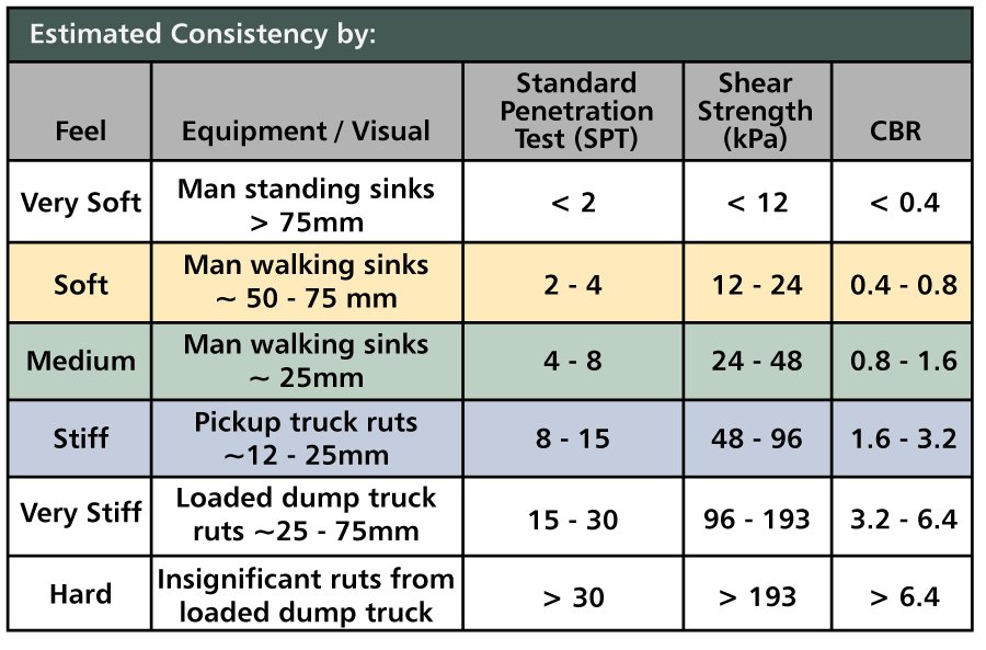
After Geotechnology for Railroaders Program, Module 2; §10. Full reference under Supplemental Sources.
Case study: 18.15.1 Chasing a CBR of 7% into competent rock (Look 2023), in §18.15 Case Studies.
The AASHTO 1993 design equation for flexible pavement structural number (SN) is:
Where:
Solve iteratively for SN given W₁₈, R, S₀, and M_r.
Reference graphics
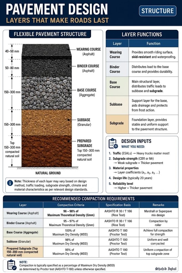
Reference graphics · click to zoom
Where:
| Layer Material | a_i | Typical D_i (in.) | Notes |
|---|---|---|---|
| Dense-graded HMA (surface/binder) | 0.44 | 4–8 | AASHTO M 320; PG 76-22 for heavy truck |
| Emulsified asphalt treated base | 0.34 | 4–8 | Used as intermediate base layer |
| Crushed aggregate base (CAB) | 0.14 | 6–12 | AASHTO M 147; CBR ≥ 80% |
| Granular subbase (GSB) | 0.11 | 6–18 | CBR ≥ 20%; used for frost protection |
| Portland cement concrete (JPCP) | — | 8–14 | Rigid design uses k/slab thickness method |
| Cement-treated base (CTB) | 0.23 | 6–10 | Unconfined compressive strength ≥ 300 psi |
| Lime-stabilized subgrade | 0.10 | 6–12 | PI reduction to < 12 |
Loaded container handler (reach stacker): 180,000 lb GVW; tandem steer axle ~50,000 lb; dual-tire drive axle ~130,000 lb.
For a 130,000-lb tandem drive axle: ESAL_factor = (130,000/32,000)^4.0 per tandem axle formula ≈ 35.7 ESALs per pass. A terminal handling 500 loaded container moves per day generates approximately:
This confirms the 10–15M ESAL design life target in Table 18-1 is appropriate for active intermodal terminals.
Where yard tracks, grade crossings or intermodal loading tracks share a paved area, the same layered-elastic logic used for pavements applies to the track. Huang, Rose and Khoury (University of Kentucky) developed a thickness method using the KENTRACK program and two criteria: horizontal tensile strain at the bottom of the HMA (fatigue cracking) and vertical compressive stress — not strain, as in highway practice — on top of the subgrade (permanent deformation).
Source: Huang, Y. H., Rose, J. G. and Khoury, C. J. (c. 1987). “Thickness Design for Hot-Mix Asphalt Railroad Trackbeds.” Proc. Association of Asphalt Paving Technologists, pp. 427–453 (scanned; text recovered by OCR)
For jointed plain concrete pavement (JPCP), the AASHTO 1993 rigid pavement design equation is:
Where:
Reference graphics
For CPKC and CN facilities in northern climates, frost penetration depth Z_f (ft) is estimated using the modified Berggren equation:
Where:
Design freezing indices by location (99% confidence level):
| Location | Design F_I (°F-days) | Typical Z_f (ft) |
|---|---|---|
| Winnipeg, MB (CPKC) | 3,800 | 7.5–9.0 |
| Edmonton, AB (CPKC/CN) | 3,200 | 6.5–8.0 |
| Thunder Bay, ON (CN) | 3,000 | 6.0–7.5 |
| Chicago, IL (BNSF/CN) | 1,200 | 3.5–4.5 |
| Minneapolis, MN (BNSF/CPKC) | 1,800 | 4.5–5.5 |
| Kansas City, MO (BNSF/CPKC) | 800 | 2.5–3.5 |
| Atlanta, GA (CSXT/NSR) | 150 | 0.5–1.0 |
Frost susceptibility is classified per the USACE system (modified for pavement applications):
| Group | Frost Susceptibility | Soil Types | Heave Rate (in./day) | Design Action |
|---|---|---|---|---|
| F0 | Negligible | GW, GP | < 0.002 | No frost protection needed |
| F1 | Low | GW, GP with fines; SW, SP | < 0.004 | Minimal protection; monitor |
| F2 | Medium | SM, GP-GM, GW-GM | 0.004–0.008 | Partial replacement with non-frost-susceptible material |
| F3 | High | SC, ML, CL, GC | 0.008–0.020 | Full replacement to Z_f or frost protection layer |
| F4 | Very High | CH, MH, OL, OC; varved clays | > 0.020 | Full replacement; subgrade stabilization; drainage mandatory |
CPKC TS and CN ES require replacement of all F3 and F4 subgrade materials within the frost depth zone with granular material meeting: P-200 ≤ 3%, CBR ≥ 40%, non-plastic.
During spring thaw, subgrade strength may be reduced to as low as 20–30% of the non-frozen value due to saturated, softened conditions. CPKC and CN apply a seasonal correction factor:
Where f_thaw = 0.20 to 0.35 (conservative range during thaw period). The AASHTO 1993 design addresses this through a weighted subgrade M_r using months of reduced strength:
This harmonic mean ensures that low-strength months govern the pavement structural design.
Mauduit, Livet and Piau summarize the French approach, which is useful where track and paved yard areas share frost-susceptible subgrade:
Source: Mauduit, C., Livet, J. and Piau, J-M. (2007). “Frost Design Method for Roadways and Railways – State of the Art in France.” In Gomes Correia, A., Momoya, Y. and Tatsuoka, F. (eds.), Design and Construction of Pavements and Rail Tracks. Taylor & Francis/Balkema
The frost index is the integral of below-freezing temperature over time (°F-days or °F-hours). It is chosen for a design return period: F2, F5, F10 or F100 correspond to a 50%, 20%, 10% or 1% chance of freezing through in a given winter. For track, the required ballast-plus-subballast thickness rises from about 20 in. at 360°F-days to over 6.6 ft at 2,900°F-days, depending on mean annual temperature (Figure 18-12). The same chart is a reasonable cross-check for granular protection under yard pavements built on frost-susceptible silts. Chapter 2, §2.5 has the full frost discussion.
Figures · click to zoom
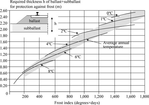
After Profillidis (2014), §9.11.1, §12.5.2, Table 9.6, Fig. 12.6. Full reference under Supplemental Sources.
Heave requires saturated soil, frost-susceptible soil (silt), sub-zero temperature, a slowly advancing freezing front, and a water supply from below. Remove any one and it stops. For yards and access roads, that means drainage that keeps the water table down and clean, low-fines granular base. Fines-rich material compacts well dry but heaves and loses strength when wet.
Figures · click to zoom
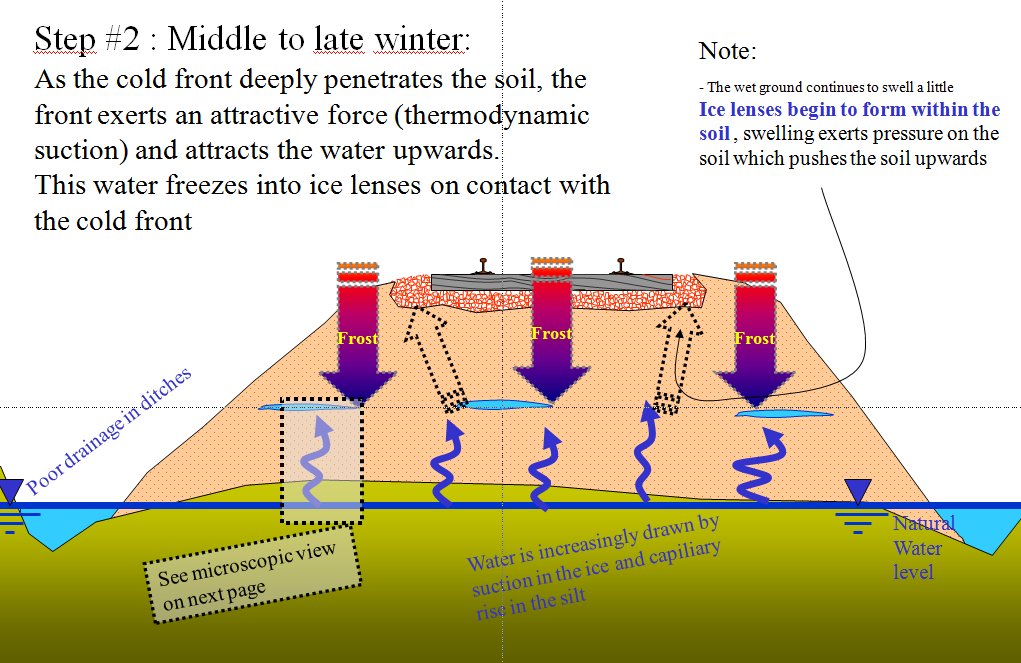
After Geotechnology for Railroaders Program, Module 6.6, Module 2; Module 6.6 §02; Module 2 §09. Full reference under Supplemental Sources.
Subgrade preparation specifications reference ASTM D698 (Standard Proctor) or ASTM D1557 (Modified Proctor):
| Railroad | Test Method | Min RC (Top 12 in.) | Min RC (Below 12 in.) | Moisture Range | Notes |
|---|---|---|---|---|---|
| UPRR | ASTM D1557 (Modified) | 95% | 92% | −2% to +2% of w_opt | Intermodal yards; Class I requirement |
| BNSF | ASTM D1557 | 95% | 92% | −2% to +2% | Heavy terminal areas |
| CSXT | ASTM D698 or D1557 | 95% (D1557) | 92% | −1% to +3% | D1557 for HMA areas |
| NSR | ASTM D698 | 95% | 90% | −1% to +3% | General yard areas |
| Amtrak | ASTM D1557 | 95% | 93% | ±2% | Station and platform areas |
| CPKC | ASTM D1557 | 98% | 95% | −2% to +1% | Frost heave mitigation |
| CN | ASTM D1557 | 98% | 95% | −2% to +1% | Prairie terminal standard |
| G&W | ASTM D698 | 95% | 90% | −1% to +3% | State DOT or AREMA |
| AREMA | ASTM D698 | 95% | 90% | ±3% | Baseline standard |
Reference graphics
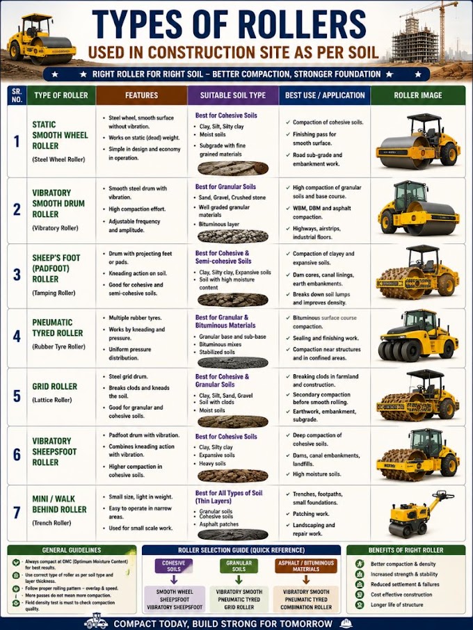
Reference graphics · click to zoom
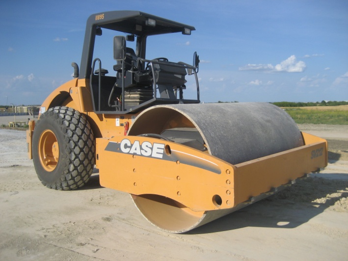
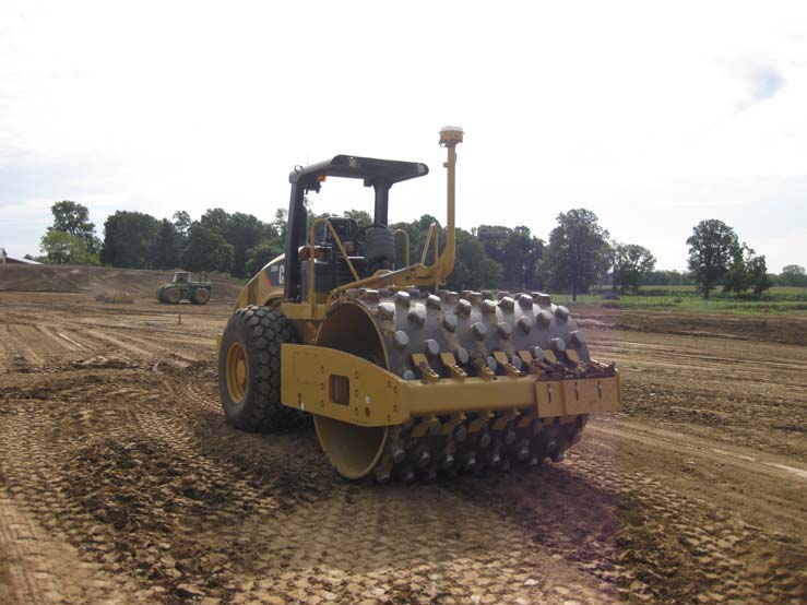
When in-situ subgrade does not meet minimum CBR or M_r criteria, stabilization options include:
Reference graphics
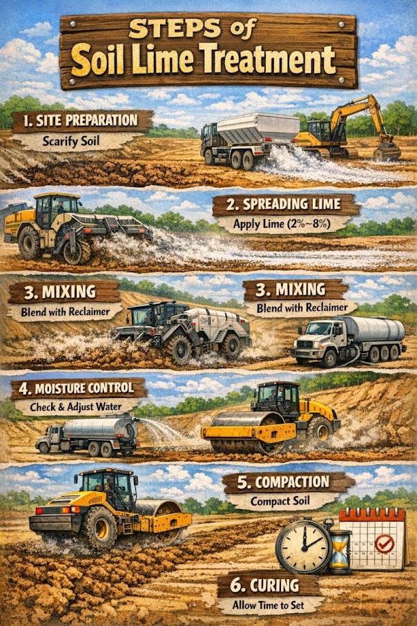
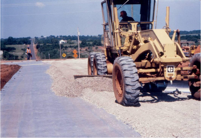
Table 18-S1. Separation vs. confinement for yard and access-road subgrades
| Geotextile separator | Geocell confinement | |
|---|---|---|
| Function | Keeps base aggregate out of soft subgrade and subgrade fines out of the base; secondary filtration, drainage, reinforcement | 3-D honeycomb (HDPE or novel polymeric alloy) confines infill, raising stiffness and strength; reduces rutting and required base thickness |
| Where it fits | Subgrade soaked CBR 3–8 (Class 2 moderate-strength geotextile); seasonally weak, high-fines or pumping-susceptible soils. Little need where the soil stays dry. | Soft to firm subgrade; most cost-effective with sand or rounded gravel infill (e.g., local material that would not otherwise qualify as base) |
| Design basis | Empirical (FHWA NHI-07-092 / AASHTO M 288 survivability, retention, permeability); separation does not reduce the base thickness needed for traffic | No FHWA method; research methods (e.g., KENLAYER damage analysis, modified Giroud–Han), modulus improvement factor capped at 7.6 for NPA cells |
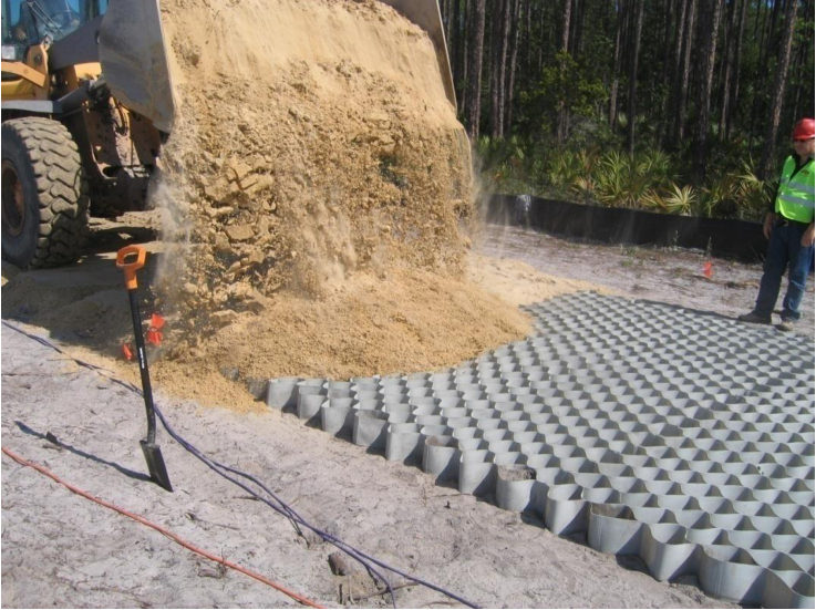
| Construction notes | End-dump base from the edge of the fabric; compact with a smooth-drum roller rather than vibratory compaction; maintain overlaps; hard to place in wind | Stretch and pin cells, usually over a nonwoven separator; fill and compact (compaction inside cells is a known difficulty) |
| Limitations | Not in AASHTO M-E; life-cycle benefit not yet demonstrated; not economical where good base is cheap | Limited design, QC/QA methods and long-term data; product cost |
For railroad use, the same separation criteria apply beneath subballast on fine-grained subgrade, and geocells are an option for access roads and laydown areas that must carry heavy equipment over weak ground (Figures 18-S1 and 18-S2).
Source: SHRP2 R02 / GeoTechTools (2012). Geosynthetic Separation in Pavement Systems — fact sheet, design guidance and photographs · SHRP2 R02 / GeoTechTools (2012). Geocell Confinement in Pavement Systems — fact sheet, design guidance and photographs
Case study: 18.15.2 Desiccation cracks cut subgrade modulus by about a third (Look 2023), in §18.15 Case Studies.
Intermodal yard overhead gantry cranes (Rubber Tired Gantry — RTG, or Rail Mounted Gantry — RMG) impose wheel loads of 75–150 kips per wheel on crane rail foundation beams. The geotechnical design challenge is controlling differential settlement between adjacent crane rail beam pile caps:
Differential settlement criterion:
For a 50-ft span between crane rail beam pile caps: ΔS_allow = 50 × 12 in. / 500 = 1.2 in. maximum differential. CN and CPKC tighten this to L/750 (0.80 in.) for high-cycle RTG operations.
Crane rail foundation design is addressed in Chapter 11 (bearing capacity) and Chapter 12 (settlement). The subgrade evaluation output for crane rail areas includes:
Case study: 18.15.3 Temporary haul road for a one-off heavy load (Look 2023), in §18.15 Case Studies.
Worked Example 18-1: AASHTO 1993 Flexible Pavement Design — BNSF Intermodal Yard, Kansas City
Project: New reach stacker lanes at BNSF Murray Yard expansion, Kansas City, MO. Design life 20 years; target reliability R = 95%.
Given:
Step 1 — Solve AASHTO equation for SN (iterative):
Trial SN = 6.0 in.:
Trial SN = 4.5 in.:
Interpolation yields SN ≈ 5.0 in. at W₁₈ = 8,000,000.
Step 2 — Layer design:
| Layer | Material | a_i | D_i (in.) | m_i | a_i D_i m_i |
|---|---|---|---|---|---|
| Surface | 4 in. HMA (PG 76-22) | 0.44 | 4.0 | 1.0 | 1.76 |
| Base | 8 in. CAB (CBR 80) | 0.14 | 8.0 | 0.90 | 1.01 |
| Subbase | 10 in. GSB (CBR 25) | 0.11 | 10.0 | 0.90 | 0.99 |
| Total SN | 3.76 |
SN = 3.76 < 5.0 — deficient. Revise:
| Layer | Material | a_i | D_i (in.) | m_i | a_i D_i m_i |
|---|---|---|---|---|---|
| Surface | 6 in. HMA | 0.44 | 6.0 | 1.0 | 2.64 |
| Base | 10 in. CAB | 0.14 | 10.0 | 0.90 | 1.26 |
| Subbase | 12 in. GSB | 0.11 | 12.0 | 0.90 | 1.19 |
| Total SN | 5.09 ✓ |
Step 3 — Subgrade improvement check:
CBR = 4% < BNSF minimum of 8% (Table 18-1). Lime-stabilize top 12 in. of CL subgrade with 5% hydrated lime → target PI_final < 12 → M_r,improved ≈ 9,000 psi → re-solve for SN:
With M_r = 9,000 psi, SN requirement drops to ≈ 4.1 in. Total construction savings from lime stabilization: reduce GSB from 12 in. to 6 in. and base from 10 in. to 8 in., saving approximately 12 in. of aggregate at ~$18/ton = $2.20/ft² savings over the terminal footprint.
Recommendation: 5% lime stabilization of subgrade + 6 in. HMA + 8 in. CAB + 6 in. GSB (SN = 4.41 in. > 4.1 in. required).
Worked Example 18-2: Rigid Pavement — CPKC Intermodal Yard, Winnipeg
Project: New RTG crane runway and reach stacker lanes, CPKC Winnipeg Intermodal Terminal expansion. Frost depth = 8.0 ft design. Design life 25 years.
Given:
Step 1 — Solve rigid pavement design equation for D (iterative):
Trial D = 11 in.:
Try D = 10 in. → verify W₁₈ ≈ 8.5M (< 12M target). D = 11 in. governs.
Recommendation: 11-in. JPCP with #5 dowel bars at 12-in. spacing at transverse joints; 15-ft joint spacing; PCC f'_c = 4,500 psi. Subgrade: full replacement of F3 material to 8.0 ft with Type A granular fill (non-frost-susceptible, P-200 ≤ 3%). Geotextile separator at subgrade interface (CPKC TS Geotextile Specification).
Worked Example 18-3: Frost Penetration and Seasonal M_r — CN Prairie Terminal
Project: CN Winnipeg North Transfer Facility, MOB access roads. Winter design required.
Given:
Step 1 — Frost depth:
Step 2 — Weighted subgrade M_r (harmonic mean, 12-month basis):
| Months | Condition | M_r (psi) |
|---|---|---|
| June–Oct (5 mo) | Summer | 5,500 |
| Nov (1 mo) | Freezing | 4,000 |
| Dec–Feb (3 mo) | Frozen | 8,000 |
| Mar (1 mo) | Early thaw | 2,000 |
| Apr–May (2 mo) | Spring thaw | 1,375 |
Step 3 — Conclusion: Design subgrade M_r = 3,440 psi (seasonal average governs over 5,500 summer value). Required SN increases by approximately 18% relative to a non-frost-corrected design — equivalent to adding 2 in. of HMA or 5 in. of granular base. CN ES requires the frost-depth granular replacement to eliminate M_r thaw reduction at critical subgrade depths.
| Sample ID | Depth (ft) | USCS | LL | PL | PI | P-200 (%) | γ_d (pcf) | w_opt (%) | CBR soaked (%) | M_r (psi) | FS Class |
|---|---|---|---|---|---|---|---|---|---|---|---|
| TP-1 / 0–2 | 0.5 | CL | 38 | 19 | 19 | 68 | 98 | 16 | 3.5 | 5,250 | F3 |
| TP-1 / 2–4 | 3.0 | CL | 41 | 20 | 21 | 72 | 96 | 18 | 3.0 | 4,500 | F3 |
| TP-2 / 0–2 | 0.5 | ML | 32 | 24 | 8 | 74 | 100 | 14 | 4.0 | 6,000 | F3 |
| TP-2 / 2–4 | 3.0 | CL | 44 | 22 | 22 | 78 | 95 | 19 | 2.5 | 3,750 | F3 |
| TP-3 / 0–2 | 0.5 | SM | 28 | 21 | 7 | 38 | 108 | 12 | 8.5 | 12,750 | F2 |
| TP-3 / 2–4 | 3.0 | SC | 35 | 18 | 17 | 52 | 102 | 15 | 5.5 | 8,250 | F3 |
| TP-4 / 0–2 | 0.5 | GC | 30 | 18 | 12 | 18 | 118 | 10 | 18 | 27,000 | F2 |
| TP-4 / 2–4 | 3.0 | GM | 26 | 16 | 10 | 22 | 116 | 11 | 15 | 22,500 | F2 |
All CBR values at Modified Proctor 95% RC, soaked 4 days per ASTM D1883. M_r estimated from CBR using Heukelom & Klomp (CBR ≤ 10) and NCHRP 1-28A (CBR > 10).
Figure 18-1: AASHTO 1993 Nomograph — SN vs. W₁₈ for varying M_r values (3,000 to 15,000 psi) at R = 95%, S₀ = 0.45, ΔPSI = 2.2. BNSF Kansas City design point plotted.
Figure 18-2: Pavement cross-section schematic — intermodal yard flexible pavement (lime-stabilized subgrade + GSB + CAB + HMA), annotated with layer thicknesses and material specifications per BNSF EI.
Figure 18-3: JPCP cross-section — CPKC Winnipeg crane runway (11-in. slab + 8-ft granular frost protection + geotextile separator + CL subgrade), with dowel bar detail at transverse joint.
Figure 18-4: CBR vs. M_r correlation chart — both Heukelom & Klomp and NCHRP 1-28A relationships plotted with laboratory data points from Table 18-7.
Figure 18-5: Frost penetration depth Z_f vs. Freezing Index F_I for k_f = 0.75, 1.00, 1.25, 1.50 BTU/hr·ft·°F — curves covering F_I range of 500–4,000 °F-days with CN and CPKC design points highlighted.
Figure 18-6: Seasonal M_r variation profile — 12-month plot of M_r(t) for CN Prairie terminal showing summer, freezing, frozen, and thaw periods with harmonic mean M_r = 3,440 psi annotated.
Figure 18-7: Intermodal yard plan view — test pit and CBR sampling layout showing reach stacker lanes, crane runway, container stacking grid, and areas of F2 vs. F3 frost susceptibility (from Table 18-7 results).
Figure 18-8: Subgrade improvement comparison — untreated CL vs. 5% lime-stabilized CL, showing PI reduction, CBR improvement, and M_r improvement with pavement SN reduction.
Figure 18-9: Container crane RTG wheel load distribution diagram — crane rail beam, pile caps, and subgrade stress bulb at 2:1 distribution showing stress at subgrade surface for 120-kip RTG wheel load.
Figure 18-10: ESAL accumulation curves — BNSF Kansas City terminal projected W₁₈ vs. years of operation for low, medium, and high throughput scenarios, with 20-yr design ESAL = 8M annotated.
Reference graphics
Reference graphics
Reference graphics · click to zoom
The only access road to Union Pacific’s Lathrop, CA intermodal facility (about 300,000 lifts/yr) was 7.5-in. unreinforced, undoweled PCC panels with corner breaks, cracking and faulting, and signs of weak subgrade. Grinding the faults would not have fixed the rocking panels. Full-depth replacement was estimated at about twice the rehabilitation budget. About 15,100 yd2 were instead rubblized in place with a multi-head breaker and overlaid with HMA within the seven-day road curfew. The authors estimate about 250% savings versus full-depth PCC for the same 20-year life. Geotechnical points from the project:
Source: Limburg, A. and Nielsen, D. (2019). “Fast-Tracked Pavement Maintenance Using Concrete Rubblization.” AREMA 2019 Annual Conference Proceedings
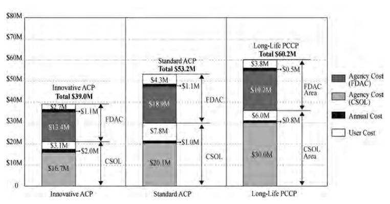
In Bull’s volume, Lee, Kim and Harvey (Chapter 4) check the pavement type chosen for Caltrans’ I-710 Long Beach rehabilitation. They follow the Caltrans life-cycle cost procedure: a 60-year analysis period, a 4% real discount rate and no salvage value. Three alternatives were compared: innovative long-life asphalt (the design actually built), standard asphalt, and long-life concrete. Two tools were used. CA4PRS estimated the construction schedule, the number of closures, and the work-zone user delay for the initial work and for every future maintenance and rehabilitation event. RealCost then discounted the agency and user costs.
Agency cost started from unit prices × quantities, taken from the contractor bid database. Allowances for traffic handling, drainage, storm-water protection, minor items, mobilization, supplemental work and a 20% contingency were then applied as cumulative multipliers. Together these multiplied the bare pavement cost by 1.80.
The closure count proved central. The built design needed 10 fifty-five-hour weekend closures at first and about 296 seven-hour night closures over 60 years. The concrete option needed 30 weekend closures at first, a further 18 at year 50, and about 148 nights.
Table 18-PM1. Table: 60-year present values (after Lee, Kim and Harvey in Bull 2015, Table 4.3)
| Alternative | Agency cost | User cost | Total |
|---|---|---|---|
| Innovative long-life AC | $33.2M | $5.8M | $39.0M |
| Standard AC | $41.1M | $12.1M | $53.2M |
| Long-life PCC | $50.4M | $9.8M | $60.2M |
The standard asphalt option had the lowest initial cost but the highest life-cycle user cost, about twice that of the design that was built.
For railroad work: for intermodal yard pavements, crane-rail runways and grade-crossing approaches, compare subgrade treatment and pavement options the way Caltrans did. For each alternative:
The same accounting applies to track itself: count the track windows each subgrade option needs over its life, not only the windows for first construction. State the markups explicitly, as the cumulative multiplier table does, so that a reviewer can see how much of the estimate is contingency.
Source: Bull, J. W. (ed.) (2015). Life Cycle Costing for the Analysis, Management and Maintenance of Civil Engineering Infrastructure. Dunbeath, Scotland: Whittles Publishing, pp. 91–108. Summarized and paraphrased; figures reproduced for internal reference. Full reference under Supplemental Sources.
Checklist · Part VIII · Pavements
Site Investigation Phase
Laboratory Testing Phase
Design Phase
Deliverable Phase
Question 10-1: A CSXT intermodal yard in Jacksonville, FL has subgrade CL with soaked CBR = 5%. Estimate M_r using the Heukelom & Klomp equation. What AASHTO 1993 SN is required for W₁₈ = 10,000,000 ESALs, R = 95%, S₀ = 0.45, ΔPSI = 2.2?
Answer 10-1:
Trial SN = 5.0: log W₁₈ = (−1.645)(0.45) + 9.36 log(6.0) − 0.20 + [log(2.2/2.7)] / [0.40 + 1094/(6.0)^5.19] + 2.32 log(7,500) − 8.07
(6.0)^5.19 = e^(5.19 × ln 6.0) = e^(5.19 × 1.792) = e^9.30 = 10,938
= −0.740 + 9.36(0.778) − 0.20 + (−0.089)/(0.40 + 0.100) + 2.32(3.875) − 8.07
= −0.740 + 7.282 − 0.20 − 0.178 + 8.990 − 8.07 = 7.084
W₁₈ = 10^7.084 = 12,140,000 (slightly high; SN = 4.8 in. governs) → SN ≈ 4.8 in.
Layer design: 5 in. HMA (SN_1 = 2.20) + 8 in. CAB (SN_2 = 0.14 × 8 × 0.90 = 1.01) + 12 in. GSB (SN_3 = 0.11 × 12 × 0.90 = 1.19) → SN_total = 4.40 in.
Revise: 6 in. HMA + 8 in. CAB + 10 in. GSB → SN = 2.64 + 1.01 + 0.99 = 4.64 in. ≈ required. Use 6–8–10 section; add lime stabilization to raise CBR from 5% to 8% target for CSXT.
Question 10-2: A CPKC Prairie facility in Regina, SK has freezing index F_I = 3,200 °F-days. Subgrade is ML (elastic silt) with w = 18%, γ_d = 102 pcf. Thermal conductivity k_f = 1.05 BTU/hr·ft·°F. Compute frost depth and frost susceptibility classification.
Answer 10-2:
Question 10-3: A reach stacker at an NSR Atlanta terminal has a tandem drive axle load of 110,000 lb. How many ESALs does one pass (loaded outbound + empty return) represent, using the 4th-power rule? If the terminal handles 300 container moves per day, what is the annual ESAL count?
Answer 10-3:
Question 10-4: A UPRR intermodal yard subgrade has M_r = 4,500 psi from laboratory testing. What is the estimated k modulus (pci) for rigid pavement design? What concrete slab thickness D is required if UPRR targets W₁₈ = 15M ESALs, R = 95%, S₀ = 0.35, S'_c = 650 psi, J = 3.2, C_d = 1.0, p_t = 2.5?
Answer 10-4:
(12)^8.46 term → 1+1.624×10⁷/(12)^8.46 ≈ 1.012 (from previous computation) log W₁₈ = −(1.645)(0.35) + 7.35 log(12) − 0.06 + (−0.079/1.012) + (4.22 − 0.80)(0.015) = −0.576 + 7.930 − 0.06 − 0.078 + 0.051 = 7.267 → W₁₈ = 18.5M D = 11 in. supports 18.5M > 15M → D = 10.5 in. (govern; specify 11 in. for constructability) UPRR recommended section: 11-in. JPCP with 6-in. CAB base, #5 dowel bars at 15-ft joints.
Question 10-5: CN geotechnical data shows a CH subgrade (CBR = 2%) beneath a proposed Thunder Bay, ON intermodal yard. AASHTO Group Index (GI) must be reported. Given: LL = 62, PL = 22, P-200 = 88%. Is this soil suitable as a subgrade material? What treatment is recommended?
Answer 10-5:
| Topic | Refer To |
|---|---|
| Soil classification (USCS and AASHTO) | Chapter 8, Sections 8.2–8.5 |
| In situ testing for M_r (PLT, DCP) | Chapter 7, Section 7.3 |
| Groundwater depth and seasonal variation | Chapter 9, Sections 9.2–9.4 |
| Bearing capacity under crane rail loads | Chapter 11, Sections 11.2–11.4 |
| Settlement under surcharge / crane loads | Chapter 12, Sections 12.3–12.5 |
| Ground improvement for subgrade upgrade | Chapter 17 |
| Subgrade compaction testing | Chapter 15, Sections 15.1–15.2 |
| Laboratory CBR, Proctor, Atterberg Limits | Chapter 10, Sections 10.2, 10.5, 10.6 |
| Report format for geotechnical pavement data | Appendix E, Section E.4 |
End of Chapter 18 — Pavement Subgrade Evaluation
Field case studies by Burt G. Look, from Earthworks: Theory to Practice – Design and Construction (CRC Press/Balkema, 2023), chosen for this chapter’s topics. Each is summarized from the book with its key figures and a closing note on railroad application added by the authors of this manual. Credit for the case material belongs to Look; see item S10 under Supplemental Sources.
Related section: 18.2 Subgrade Strength Testing
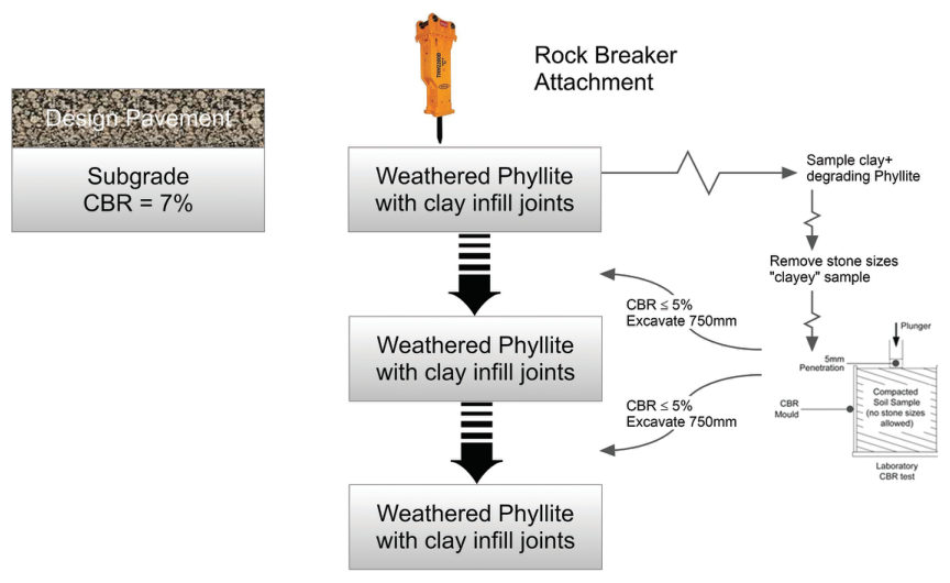
Urban road works at Kelvin Grove, Brisbane (2002) required a soaked subgrade CBR of 7% over residual soil and near-surface phyllite. The weathered rock at subgrade level degraded to soil after rain. Samples were taken from the degraded surface with its clay seams, and the laboratory removed the “stone” sizes. The CBR came back at 5% or less. Two further rounds of excavation, each needing a rock-breaker attachment to reach the next sample depth, also failed, ending 4.9 ft below design level, with about AU$100,000 of claims for “unsuitable subgrade” and delays in a busy urban area.
Look’s review found that only the top 4 in had degraded. Below it was competent rock (it needed a rock breaker) with a CBR well above 10%, and once the pavement covered it no further degradation would occur. The tests themselves were unrepresentative because the stone fraction was discarded, so the low CBR could be disregarded.
For railroad work: the same cycle can play out under a new track or yard pavement in weathered shale or phyllite. Protect the formation from rain, trim the softened skin, and check whether the sample is representative before ordering more over-excavation.
Source: Look, B. G. (2023). Earthworks: Theory to Practice – Design and Construction. CRC Press/Balkema. Case study §6.11, pp. 192–194. Summarized and paraphrased; figures reproduced for internal reference. Full reference under Supplemental Sources.
Related section: 18.6 Subgrade Preparation and Compaction Criteria
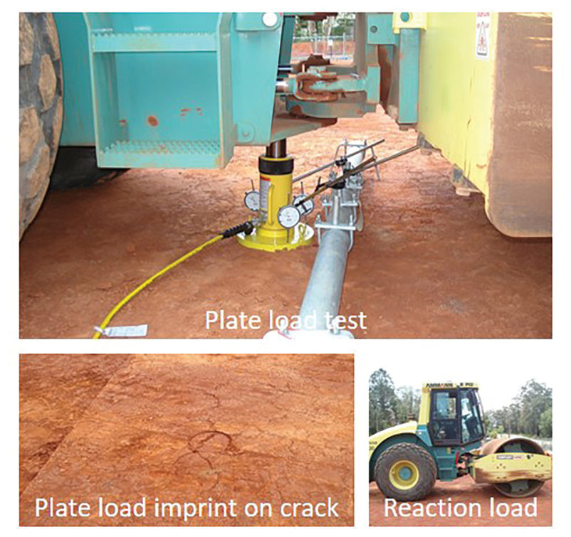
An expansive clay subgrade passed its density tests (above 95% standard MDD) and was then left uncovered for several weeks of wind and heat. Desiccation cracks appeared, and the question was whether the design modulus of 7,200 psi (CBR about 5%) still held. Plate load tests on cracked and uncracked areas, using the site roller as reaction, showed the cracked areas reached about 60% of the uncracked modulus on the first load cycle and 70% on the second, which is used for fill. The target was EV2 above 7,200 psi at formation level and above 4,350 psi below it. A one-third loss of strength or modulus is typical for fissured or desiccated clays in design.
Table 18-LK1. Plate load tests on uncracked and cracked compacted clay (after Look 2023, Table 10.18)
| Load cycle | Uncracked E (psi) | Cracked E (psi) | Ratio |
|---|---|---|---|
| First | 4,600 | 2,760 | ~60% |
| Second | 11,600 | 8,100 | 70% |
For railroad work: a finished clay subgrade awaiting subballast should be covered or kept moist. If it cracks, re-test it before placing subballast; a passing density test from before the drying no longer applies.
Source: Look, B. G. (2023). Earthworks: Theory to Practice – Design and Construction. CRC Press/Balkema. Case study §10.16, pp. 366–368. Summarized and paraphrased; figures reproduced for internal reference. Full reference under Supplemental Sources.
Related section: 18.7 Intermodal Yard Crane Rail Foundation Subgrade
Wind-farm and substation access roads may carry a single heavy delivery, where a bogged transporter can cost over a million dollars. A 22-ton or 44-ton axle exerts about 92 or 116 psi at the running surface. These are wheeled loads, so the BR470 working-platform method for tracked plant does not apply, and neither does ordinary road pavement design; the Giroud and Han (2004) method is typically used. Roads and hardstands typically need 5,200 and 6,300 psf allowable bearing, more on grades above about 5%.
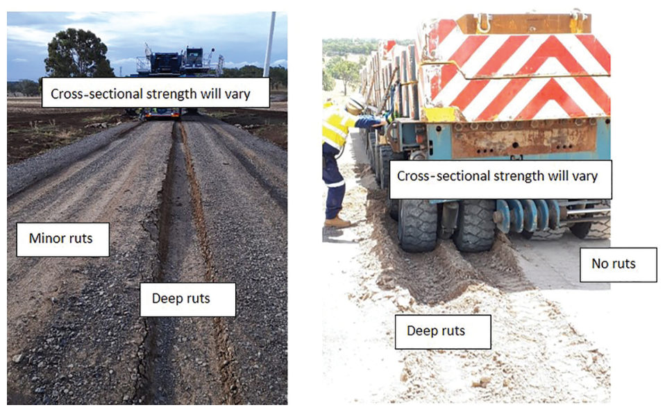
Soaked tests and drainage are usually left out of a one-off design for cost reasons, so rain is the main risk: Look treats more than about 0.8 in of rain as high risk when an unsoaked CBR was used. At this site the proof roll failed the day before the move, after 2.1 in. and 1.1 in. of rain two and three days earlier. No passing proof roll was seen, but the equipment went on anyway, with significant consequences. Deep ruts under one wheel and none under the other showed non-uniform construction or support.
Recommended field data: DCP, vane shear, light falling-weight deflectometer and plate load tests, with plate tests kept to hardstands and critical spots. The maximum plate pressure reached is not the allowable bearing capacity. In one example a 1,250 psf design subgrade strength, with influence extending 24–31 in, gave calculated ruts above 2 in.
Table 18-LK2. Ground contact pressure by axle load (after Look 2023, Table 11.5)
| Axle load (tons) | Wheel load (tons) | Contact area (in.²) | Contact pressure |
|---|---|---|---|
| 13 | 6.6 | 167 | 80 psi |
| 22 | 17 | 240 | 92 psi |
| 44 | 22 | 380 | 116 psi |
For railroad work: the same logic applies to crane pads and temporary access for bridge erection, transformer delivery to traction substations and intermodal heavy lifts. Hold the move on a failed proof roll after rain.
Source: Look, B. G. (2023). Earthworks: Theory to Practice – Design and Construction. CRC Press/Balkema. Case study §11.7, pp. 390–392. Summarized and paraphrased; figures reproduced for internal reference. Full reference under Supplemental Sources.
Authors: Daniel P. Colwell and Mario Ruel. This chapter was written and compiled by Daniel P. Colwell and Mario Ruel for Railway Ground Hazard Risk Management.
Technical content is drawn from the published sources below, and credit for that material belongs to their authors and publishers. Tables, equations and figures taken from a specific source are also cited where they appear.
File locations for these documents are listed under Supplemental Sources — LEVI Library.
Material in the green “Supplemental reference” boxes throughout this chapter was added from the following documents in the LEVI geotechnical library. Text is summarized or paraphrased; tables are reproduced with their original source noted; figures are reproduced from the cited document for internal reference use. Consult the original document before relying on a value for design. Blocks marked “After Selig & Waters (1994)” summarize item S9 for railroad clients; tables are condensed from the book and its figures are not reproduced. The Case Studies section summarizes case studies from item S10 by Burt G. Look; its figures are reproduced from the book for internal reference use, and the closing “For railroad work” note in each case study is added by the authors of this manual. Blocks tagged “Project management” summarize methods, examples and figures from the project-management, estimating and construction-management books listed here, applied to railroad work; the closing “For railroad work” note in each block is added by the authors of this manual.